Everybody herds, sometimes: cumulative advantage as a product of rational learning

Figures & data

Figure 1. Proportions of agents staying with their object of choice given that it failed (${\epsilon }_0\left(\mathit{n}\right)$) on the y-axis by round on the x-axis; gray lines depict 100 runs for each neighborhood size k, black lines plot means per round; agents learn optimally.

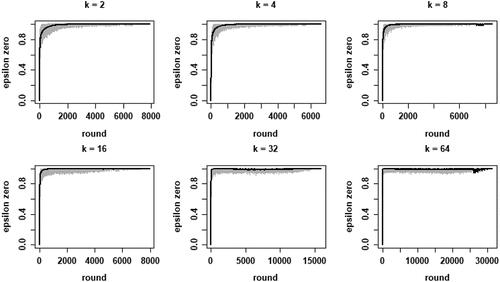
Figure 2. Mean proportions of agents staying with their object of choice given that it failed (${\epsilon }_0\left(\mathit{n}\right)$) on the y-axis by round on the x-axis; 100 runs for each neighborhood size k; black = 2 neighbors, blue = 4 neighbors, red = 8 neighbors, green = 16 neighbors, yellow = 32 neighbors, orange = 64 neighbors; agents learn optimally.

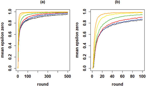
Figure 3. Boxplots of the distributions of Gini coefficients of the distribution of agent choices among high quality objects; Gini coefficients of 100 runs at convergence, per value of k.

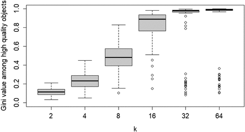
Figure 4. Boxplots of total search costs until convergence (based on Eq. (5) summed over all rounds n per run) for all values of k; y-axis running from 0 to 350 for k equal to 2, 4, and 8, from 0 to 8000 for k equal to 16 and 32, and from 0 to 20,000 for k equal to 64.

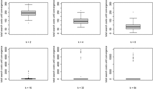
Figure 5. Proportions of agents converging on high quality (HQ) object for each value of ${\epsilon }_0$, for all values of k; 20 runs per value of ${\epsilon }_0$; solid lines depict mean proportions; dots are jittered for better representation.

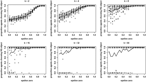
Figure 6. Gini coefficient values among high quality (HQ) objects in terms of numbers of agents choosing objects for each value of ${\epsilon }_0$, for all values of k; 20 runs per value of ${\epsilon }_0$; data for runs that have at least one agent converging on an HQ object; solid lines depict mean Gini.

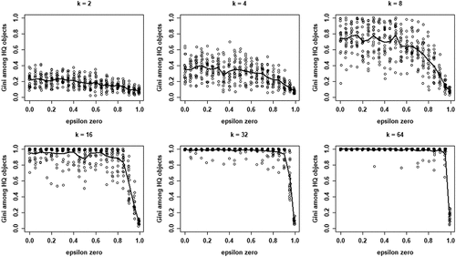
Figure 7. Search costs according to Eq. (5) for different values of ${\epsilon }_0$, for each values of k; runs that end in all agents converging on a HQ object only.

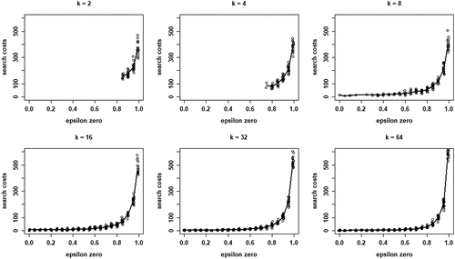
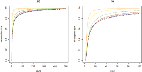
Figure 8. Average outcomes of learning under the common knowledge of rationality assumption; the left panel shows mean search costs, the right panel shows mean Gini coefficients. Neighborhood sizes: black for k = 2, blue for k = 4, red for k = 8, green for k = 16, yellow for k = 32, and orange for k = 64.

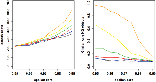
Figure 9. Proportions of agents staying with their object of choice given that it failed (${\epsilon }_0\left(\mathit{n}\right)$) on the y-axis by round on the x-axis; gray lines depict 100 runs, blue lines plot means per round; the optimal learning scenario is depicted in the left-hand plot and the “most promising” common knowledge scenario in the right-hand plot.

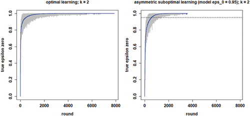
Figure B1. Search costs according to Eq. (5) for different values of ${\epsilon }_0$, for each values of k; all runs.

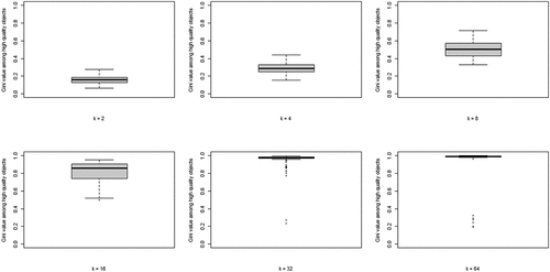
Figure B2. Proportions of agents choosing a HQ object at convergence for different values of $\mathit{\epsilon }$, for each value of neighborhood size k; solid lines are mean proportions.

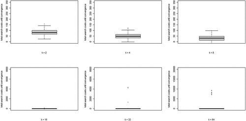
Figure B3. Gini coefficient values among HQ objects for different values of $\mathit{\epsilon }$, for all values of k.

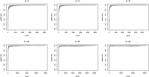
Figure B4. Search costs according to Eq. (5)(5) $\mathit{s}\left(\mathit{n}\right)=1-\frac{\mathit{p}\left(\mathit{n}\right)-\mathit{pL}}{\mathit{pH}-\mathit{pL}}$(5) for different values of $\mathit{\epsilon }$ across all runs for each value of k.

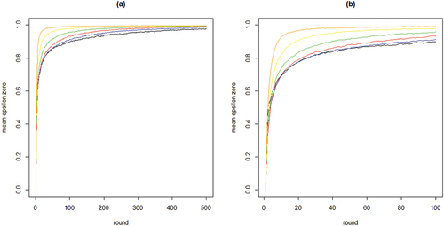
Figure B5. Search costs according to Eq. (5)(5) $\mathit{s}\left(\mathit{n}\right)=1-\frac{\mathit{p}\left(\mathit{n}\right)-\mathit{pL}}{\mathit{pH}-\mathit{pL}}$(5) for different values of $\mathit{\epsilon }$ for runs ending in all agents converging on a high-quality object only, for all values of k.

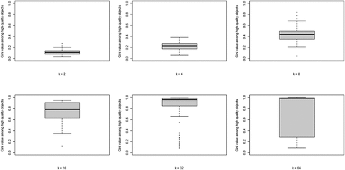
Figure B6. Box-plots of search costs in the optimal learning condition (left-hand) and the “most promising” common knowledge condition; neighborhood size k equals 2.

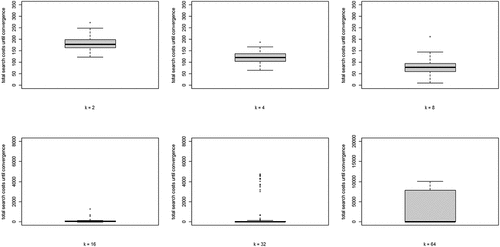
Figure B7. Boxplots if Gini coefficients at convergence in the optimal learning condition (left-hand) and the “most promising” common knowledge condition; neighborhood size k equals 2.

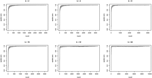
Table C1. Parameter values for robustness checks.

Robustness Check (RC)	Value of h	Value of $\left(p_L,p_H\right)$	OR
Model from paper	5	$\left(\frac{3}{4},\frac{4}{5}\right)$	$\frac{4}{3}$
RC0	10	$\left(\frac{3}{4},\frac{4}{5}\right)$	$\frac{4}{3}$
RC1a	5	$\left(\frac{1}{3},\frac{2}{5}\right)$	$\frac{4}{3}$
RC1b	10	$\left(\frac{1}{3},\frac{2}{5}\right)$	$\frac{4}{3}$
RC2a	5	$\left(\frac{3}{5},\frac{4}{5}\right)$	$\frac{8}{3}$
RC2b	10	$\left(\frac{3}{5},\frac{4}{5}\right)$	$\frac{8}{3}$
RC3a	5	$\left(\frac{1}{5},\frac{2}{5}\right)$	$\frac{8}{3}$
RC3b	10	$\left(\frac{1}{5},\frac{2}{5}\right)$	$\frac{8}{3}$

Figure C.1.1. Proportions of agents staying with their object of choice given that it failed (${\epsilon }_0\left(\mathit{n}\right)$) on the y-axis by round on the x-axis; gray lines depict 100 runs for each neighborhood size k, black lines plot means per round; agents learn optimally; RC0.

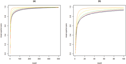
Figure C.1.2. Mean proportions of agents staying with their object of choice given that it failed (${\epsilon }_0\left(\mathit{n}\right)$) on the y-axis by round on the x-axis; 100 runs for each neighborhood size k; black = 2 neighbors, blue = 4 neighbors, red = 8 neighbors, green = 16 neighbors, yellow = 32 neighbors, orange = 64 neighbors; agents learn optimally; RC0.

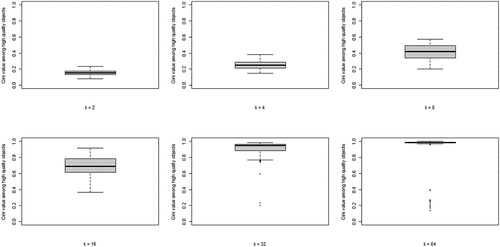
Figure C.1.3. Boxplots of the distributions of Gini coefficients of the distribution of agent choices among high quality objects; Gini coefficients of 100 runs at convergence, per value of k; agents learn optimally; RC0.

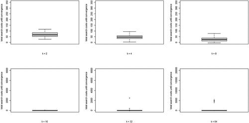
Figure C.1.4. Boxplots of total search costs until convergence (based on equation (5) summed over all rounds n per run) for all values of k; y-axis running from 0 to 350 for k equal to 2, 4, and 8, from 0 to 8000 for k equal to 16 and 32, and from 0 to 20,000 for k equal to 64; agents learn optimally; RC0.

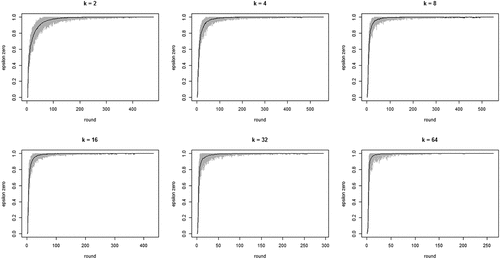
Figure C.2.1. Proportions of agents staying with their object of choice given that it failed (${\epsilon }_0\left(\mathit{n}\right)$) on the y-axis by round on the x-axis; gray lines depict 100 runs for each neighborhood size k, black lines plot means per round; agents learn optimally; RC1a.

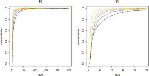
Figure C.2.2. Mean proportions of agents staying with their object of choice given that it failed (${\epsilon }_0\left(\mathit{n}\right)$) on the y-axis by round on the x-axis; 100 runs for each neighborhood size k; black = 2 neighbors, blue = 4 neighbors, red = 8 neighbors, green = 16 neighbors, yellow = 32 neighbors, orange = 64 neighbors; agents learn optimally; RC1a.

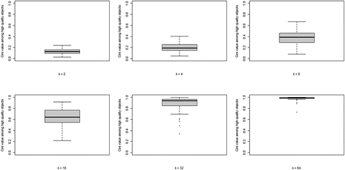
Figure C.2.3. Boxplots of the distributions of Gini coefficients of the distribution of agent choices among high quality objects; Gini coefficients of 100 runs at convergence, per value of k; agents learn optimally; RC1a.

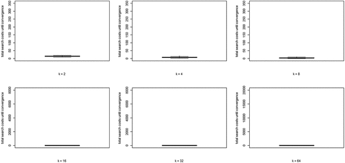
Figure C.2.4. Boxplots of total search costs until convergence (based on Eq. (5)(5) $\mathit{s}\left(\mathit{n}\right)=1-\frac{\mathit{p}\left(\mathit{n}\right)-\mathit{pL}}{\mathit{pH}-\mathit{pL}}$(5) summed over all rounds n per run) for all values of k; y-axis running from 0 to 350 for k equal to 2, 4, and 8, from 0 to 8000 for k equal to 16 and 32, and from 0 to 20,000 for k equal to 64; agents learn optimally; RC1a.

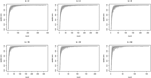
Figure C.3.1. Proportions of agents staying with their object of choice given that it failed (${\epsilon }_0\left(\mathit{n}\right)$) on the y-axis by round on the x-axis; gray lines depict 100 runs for each neighborhood size k, black lines plot means per round; agents learn optimally; RC1b.

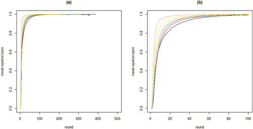
Figure C.3.2. Mean proportions of agents staying with their object of choice given that it failed (${\epsilon }_0\left(\mathit{n}\right)$) on the y-axis by round on the x-axis; 100 runs for each neighborhood size k; black = 2 neighbors, blue = 4 neighbors, red = 8 neighbors, green = 16 neighbors, yellow = 32 neighbors, orange = 64 neighbors; agents learn optimally; RC1b.

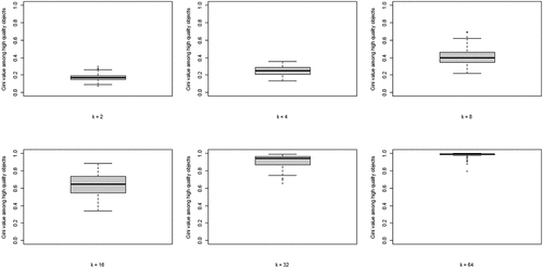
Figure C.3.3. Boxplots of the distributions of Gini coefficients of the distribution of agent choices among high quality objects; Gini coefficients of 100 runs at convergence, per value of k; agents learn optimally; RC1b.

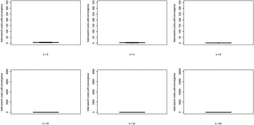
Figure C.3.4. Boxplots of total search costs until convergence (based on Eq. (5)(5) $\mathit{s}\left(\mathit{n}\right)=1-\frac{\mathit{p}\left(\mathit{n}\right)-\mathit{pL}}{\mathit{pH}-\mathit{pL}}$(5) summed over all rounds n per run) for all values of k; y-axis running from 0 to 350 for k equal to 2, 4, and 8, from 0 to 8000 for k equal to 16 and 32, and from 0 to 20,000 for k equal to 64; agents learn optimally; RC1b.

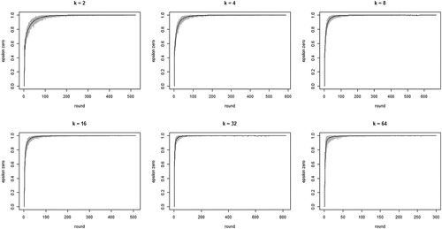
Figure C.4.1. Proportions of agents staying with their object of choice given that it failed ()on the y-axis by round on the x-axis; gray lines depict 100 runs for each neighborhood size k, black lines plot means per round; agents learn optimally; RC2a.

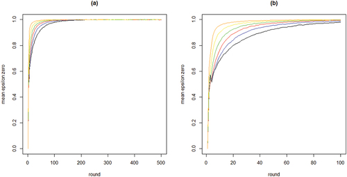
Figure C.4.2. Mean proportions of agents staying with their object of choice given that it failed (${\epsilon }_0\left(\mathit{n}\right)$) on the y-axis by round on the x-axis; 100 runs for each neighborhood size k; black = 2 neighbors, blue = 4 neighbors, red = 8 neighbors, green = 16 neighbors, yellow = 32 neighbors, orange = 64 neighbors; agents learn optimally; RC2a.

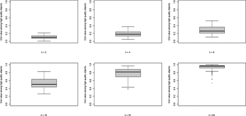
Figure C.4.3. Boxplots of the distributions of Gini coefficients of the distribution of agent choices among high quality objects; Gini coefficients of 100 runs at convergence, per value of k; agents learn optimally; RC2a.

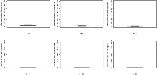
Figure C.4.4. Boxplots of total search costs until convergence (based on Eq. (5)(5) $\mathit{s}\left(\mathit{n}\right)=1-\frac{\mathit{p}\left(\mathit{n}\right)-\mathit{pL}}{\mathit{pH}-\mathit{pL}}$(5) summed over all rounds n per run) for all values of k; y-axis running from 0 to 350 for k equal to 2, 4, and 8, from 0 to 8000 for k equal to 16 and 32, and from 0 to 20,000 for k equal to 64; agents learn optimally; RC2a.

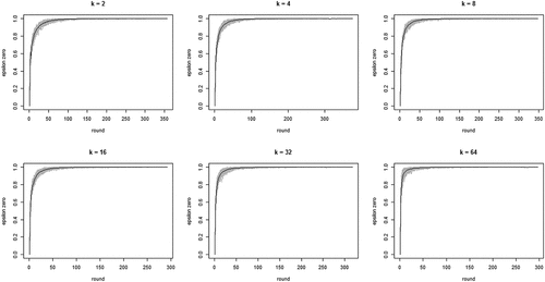
Figure C.5.1. Proportions of agents staying with their object of choice given that it failed (${\epsilon }_0\left(\mathit{n}\right)$) on the y-axis by round on the x-axis; gray lines depict 100 runs for each neighborhood size k, black lines plot means per round; agents learn optimally; RC2b.

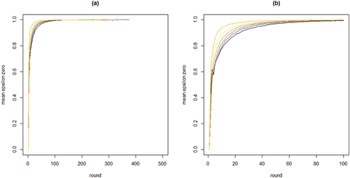
Figure C.5.2. Mean proportions of agents staying with their object of choice given that it failed (${\epsilon }_0\left(\mathit{n}\right)$) on the y-axis by round on the x-axis; 100 runs for each neighborhood size k; black = 2 neighbors, blue = 4 neighbors, red = 8 neighbors, green = 16 neighbors, yellow = 32 neighbors, orange = 64 neighbors; agents learn optimally; RC2b.

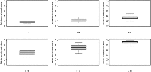
Figure C.5.3. Boxplots of the distributions of Gini coefficients of the distribution of agent choices among high quality objects; Gini coefficients of 100 runs at convergence, per value of k; agents learn optimally; RC2b.

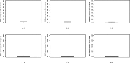
Figure C.5.4. Boxplots of total search costs until convergence (based on Eq. (5)(5) $\mathit{s}\left(\mathit{n}\right)=1-\frac{\mathit{p}\left(\mathit{n}\right)-\mathit{pL}}{\mathit{pH}-\mathit{pL}}$(5) summed over all rounds n per run) for all values of k; y-axis running from 0 to 350 for k equal to 2, 4, and 8, from 0 to 8000 for k equal to 16 and 32, and from 0 to 20,000 for k equal to 64; agents learn optimally; RC2b.

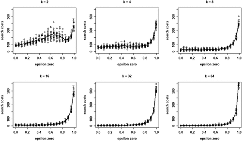
Figure C.6.1. Proportions of agents staying with their object of choice given that it failed (${\epsilon }_0\left(\mathit{n}\right)$) on the y-axis by round on the x-axis; gray lines depict 100 runs for each neighborhood size k, black lines plot means per round; agents learn optimally; RC3a.

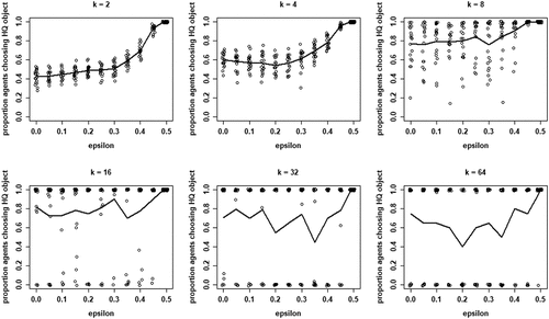
Figure C.6.2. Mean proportions of agents staying with their object of choice given that it failed (${\epsilon }_0\left(\mathit{n}\right)$) on the y-axis by round on the x-axis; 100 runs for each neighborhood size k; black = 2 neighbors, blue = 4 neighbors, red = 8 neighbors, green = 16 neighbors, yellow = 32 neighbors, orange = 64 neighbors; agents learn optimally; RC3a.

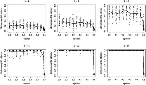
Figure C.6.3. Boxplots of the distributions of Gini coefficients of the distribution of agent choices among high quality objects; Gini coefficients of 100 runs at convergence, per value of k; agents learn optimally; RC3a.

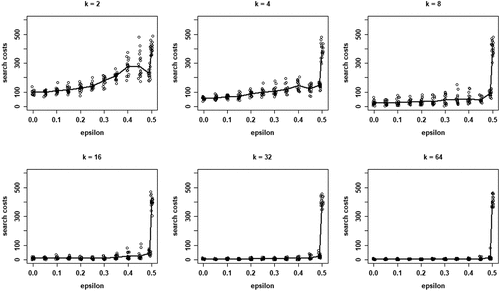
Figure C.6.4. Boxplots of total search costs until convergence (based on Eq. (5)(5) $\mathit{s}\left(\mathit{n}\right)=1-\frac{\mathit{p}\left(\mathit{n}\right)-\mathit{pL}}{\mathit{pH}-\mathit{pL}}$(5) summed over all rounds n per run) for all values of k; y-axis running from 0 to 350 for k equal to 2, 4, and 8, from 0 to 8000 for k equal to 16 and 32, and from 0 to 20,000 for k equal to 64; agents learn optimally; RC3a.

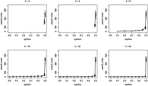
Figure C.7.1. Proportions of agents staying with their object of choice given that it failed (${\epsilon }_0\left(\mathit{n}\right)$) on the y-axis by round on the x-axis; gray lines depict 100 runs for each neighborhood size k, black lines plot means per round; agents learn optimally; RC3b.

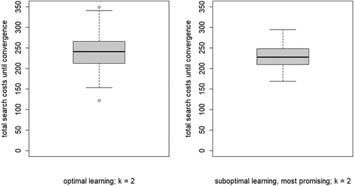
Figure C.7.2. Mean proportions of agents staying with their object of choice given that it failed (${\epsilon }_0\left(\mathit{n}\right)$) on the y-axis by round on the x-axis; 100 runs for each neighborhood size k; black = 2 neighbors, blue = 4 neighbors, red = 8 neighbors, green = 16 neighbors, yellow = 32 neighbors, orange = 64 neighbors; agents learn optimally; RC3b.

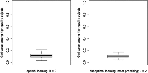
Figure C.7.3. Boxplots of the distributions of Gini coefficients of the distribution of agent choices among high quality objects; Gini coefficients of 100 runs at convergence, per value of k; agents learn optimally; RC3b.

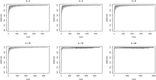
Figure C.7.4. Boxplots of total search costs until convergence (based on Eq. (5)(5) $\mathit{s}\left(\mathit{n}\right)=1-\frac{\mathit{p}\left(\mathit{n}\right)-\mathit{pL}}{\mathit{pH}-\mathit{pL}}$(5) summed over all rounds n per run) for all values of k; y-axis running from 0 to 350 for k equal to 2, 4, and 8, from 0 to 8000 for k equal to 16 and 32, and from 0 to 20,000 for k equal to 64; agents learn optimally; RC3b.