
Figures & data
Table 1. Annual population change in the United States, 2011–2015.
Figure 1. Net migrant count, net migration rate, and migration imbalance index by state.
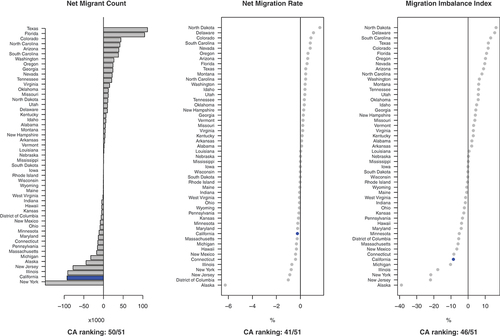
Figure 2. Quantiles of attributes for California counties (boxes) and the state as a whole (blue dots) relative to all U.S. counties. The horizontal line is the 0.5 reference line.
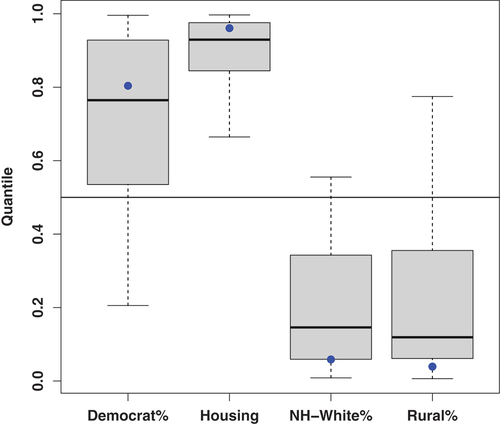
Table 2. Valued ERGM for inter-county migration flows, 2011–2015.
Figure 3. Function forms for political, racial, rural, and housing effects.
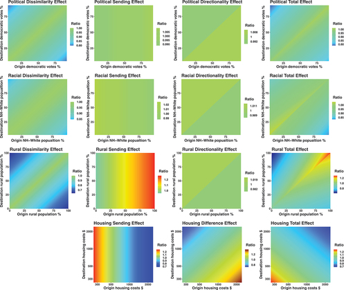
Figure 4. Function forms for migration effects involving San Francisco county. (left) dyadic effects, with vertical and horizontal lines showing SF attributes. (center) net immigration (solid lines) and emigration (dotted lines) effects for SF, given origin/destination county attributes; vertical line shows SF position. (right) areas between curves (net immigration) from the center plot by origin/destination county attributes; histograms show population-weighted distributions of U.S. counties, with brown columns indicating population in net SF-immigration counties.
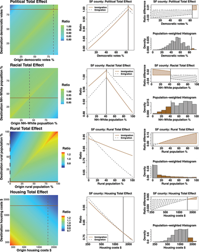
Table 3. California’s average simulated ranking with and without knockouts, by metric.
Table A1. Valued ERGM for inter-county migration flows, 2011–2015 (full model).