Figures & data
Figure 1. The experimental set-up. The subject placed his or her preferred index finger on a force sensor, and lifted it briefly whenever he or she heard a tone. In the constrained block of trials there was a straw above the finger that the subject had to be careful not to hit. In the unconstrained block of trials there was no such straw. We measured movements of the finger using a marker attached to the nail of the finger, and measured contact force using the force sensor that the finger was resting on.
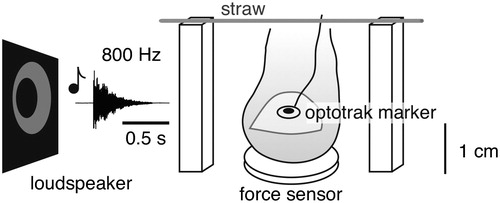
Figure 2. Determining the reaction time from the marker’s vertical positions and the vertical contact forces for one example trial. The left part shows the unsmoothed signals (position and force) and measures based on these signals (velocity, acceleration and force rate). The right side shows the same measures after smoothing the signals with a Butterworth filter at 25 Hz. Time is defined with respect to tone onset. The grey dotted line intersecting the raw position trace is the 0.5 mm displacement threshold of the simulated button. The vertical lines below the traces indicate the reaction times according to the different ways of determining the reaction time (color coded). Note how the different measures and methods give rise to quite diverse reaction times.
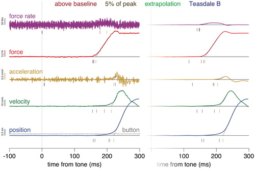
Figure 3. Distribution of reaction times for the five measures, three averaging methods and four ways of determining the RT, after smoothing the data with a Butterworth filter. Combined data for all subjects in both the constrained and unconstrained conditions. When relevant, the “button” data are also shown for comparison. Top graphs: the fractions of encountered reaction times that were shorter or equal to the value on the horizontal axis. Bottom graphs: smoothed fractions of trials for each value of the reaction time. The numbers in the top graphs give the median reaction time in ms.
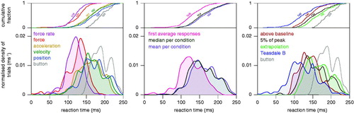
Figure 4. Standard deviation of the reaction times of the bootstrapped data for each combination of the five measures, three averaging options, three smoothing options and four ways of determining the reaction time. Combinations for which the mean reaction time was less than 50 ms are indicated by a grey background. This figure shows that first averaging the responses (pink bars) usually gives the most robust judgments of the reaction time. Combined data for all subjects in both the constrained and unconstrained conditions. The first six bars after the grey background on the left represent applying the extrapolation method to the force or position measurements, with or without either of the smoothing options.
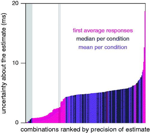
Figure 5. Extent to which averaging differently or smoothing differently results in a different estimate of the reaction time. Left: difference between the reaction time judged on the basis of the mean response and the median of the reaction times based on responses in individual trials. Right: difference between reaction times based on the raw data, data smoothed with a Butterworth filter, and data smoothed by fitting a polynomial (mean of the three possible differences). In both cases, mean values are shown for each measure and way to determine the reaction time (three standard deviations above baseline, 5% of peak amplitude, extrapolation method, Teasdale’s method B). The values are root mean squares of the differences, averaged across the constrained and unconstrained conditions (with and without straw) and the nine subjects.
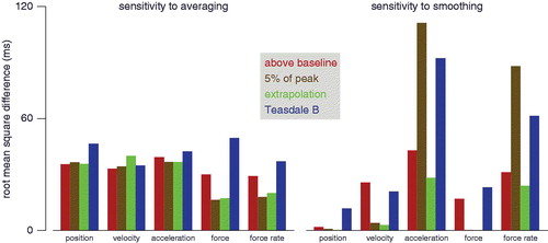
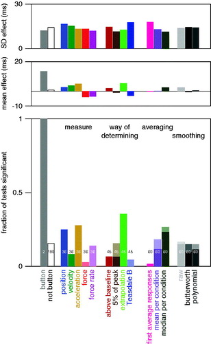
Figure 6. Extent to which different methods would lead to different conclusions. Bottom panel: fraction of options for which a t-test would lead to the conclusion that constraining the movement influences the reaction time. The numbers indicate the number of options that are considered. For the ‘button’ there are two options: taking the mean or the median of the values for each subject. The remaining options (not button) consist of all 180 combinations of the five measures, four ways of determining the reaction time, three ways of averaging, and three ways of smoothing. Pale areas at the tops of the bars (filling the whole bar for the force, force rate and Teasdale B bars) indicate that responses were significantly earlier when the movement was constrained. Middle panel: average magnitude of the effect (how much longer is the reaction time for constrained movements). Top panel: average standard deviation of the magnitude of the effect.