Figures & data
Figure 1. Mass attenuation coefficients of iodine and acrylic as a function of photon energy, as well as the calculated X-ray energy spectra with the tube voltages 80 (thin line) and 120 (thick line) kV.
Figure 2. Schematic of two-dimensional transXend detector made from a thermo-luminescent plate and two types of strip absorbers. X-rays with four different energy spectra enter the thermo-luminescent plate after passing through (α) the air, (β) absorber A, (γ) absorber B, and (δ) absorbers A and B.
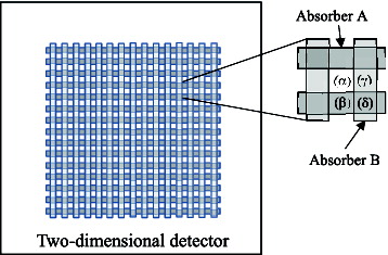
Figure 3. Calculated X-ray energy spectra for tube voltage of 120 kV after passing through the air (thick solid line), 0.1-mm-thick tin (thin solid line), 0.1-mm-thick copper (thick broken line) and both 0.1-mm-thick tin and copper (thin broken line).
Figure 4. Thermo-luminescence image. The black area in the center corresponds to the iodine region in the acrylic phantom.
Table 1. Assigned energy ranges. Emax is described in the text.
Figure 5. CT images obtained by (a) energy-resolved CT with X-rays in the energy range E2, and (b) current CT. The tube voltage was 150 kV. The CT values are shown in terms of the linear attenuation coefficient (cm−1).
Figure 6. CT value profiles obtained by energy-resolved CT and current CT with tube voltages of 100 (solid line), 120 (broken line) and 150 (dotted line) kV. Current CT results are shown as negative values for clear comparison. The CT values are shown in terms of the linear attenuation coefficient (cm−1).
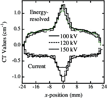
Figure 7. Summary of the CT values of acrylic (squares), iodine (circles) measured by energy-resolved (solid) and current (open) CT methods. The CT values are shown in terms of the linear attenuation coefficient (cm−1).