Simulation of melt jet breakup experiments by JASMINE with an empirical correlation for melt particle size distribution

Figures & data

Figure 1. Modeling of melt jet breakup in JASMINE code [9].

Figure 2. A simple non-local radiation heat transfer model.

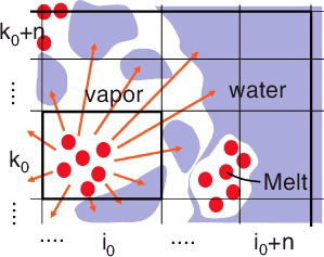
Figure 3. Treatment of settled particle groups.

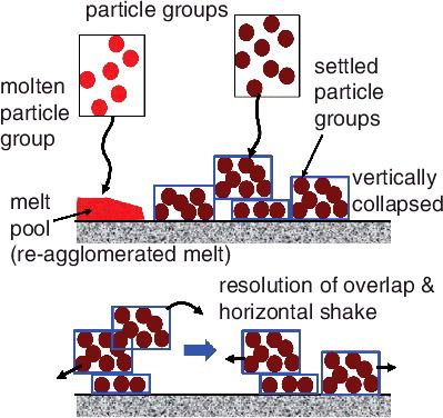
Table 1. Summary of conditions and results of selected ALPHA/GPM experiments [12].

GPM #	10	05	12	09	08
Melt material	ZAO^*1	ZAO	ZAO	SUS^*2	SUS
mass (kg)	30	30	30	70	70
Melt T (K) (superheat)	2270 (70)	2275 (75)	2280 (80)	1820 (220)	1810 (210)
Water T (K) (subcool)	344 (29)	347 (26)	373 (0)	344 (29)	371 (2)
Pool depth (m)	2.1	0.6	2.1	2.1	2.1
Jet breakup length (m)	1.2–1.25	–	1.3–1.35	1.60	∼2.0
Agglomerate fraction (%)	0	22	0	28	4.3
Debris MMD^*3(mm)	7.3	5.9	4.8	4.5	2.8
Final pool T^*4 (K)	354–367	373	373	363–365	373

Notes: System P = 0.1 MPa; melt release diameter = 33 mm; melt free fall height = 2.84 m.

^*1ZrO₂–Al₂O₃ mixture (49:51 wt%); ^*2304 stainless steel + carbon (∼5 wt%); ^*3mass median diameter; ^*4temperatures in the pool at 50—100 s (depending on cases) after the start of melt release showing stable values.

Bold lettering indicates specific differences from the base case, #10.

Figure 4. Analytical grid for ALPHA/GPM simulation (left: deep pool, right: shallow pool).

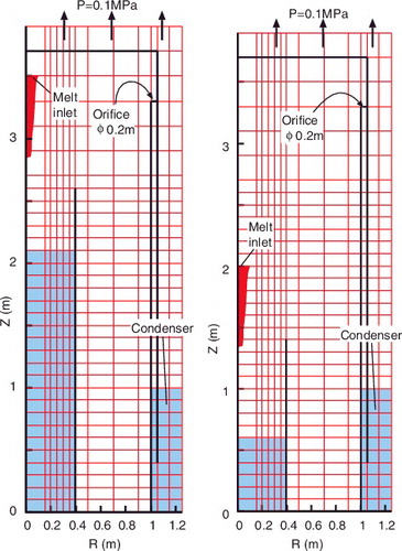
Table 2. Physical properties of the melt material used in the simulation [3,12,28,29].

	ZAO^*1	SUS^*2	Corium^*3
Liquidus/solidus temperature (K)	2200/2163	1600/1410	2850/2830
Density (liq/sol) (kg/m^3)	3360/4620	6800/6690	7960/9430
Specific heat (liq/sol) (J/kg K)	1020/970	876/831	565/445
Latent heat of fusion (MJ/kg)	1.32	0.270	0.362
Surface tension (liq) (N/m)	0.619	1.68	0.45
Emissivity	0.47	0.80 (oxide)	0.79

^*1ZrO₂–Al₂O₃ mixture (49:51 wt%); ^*2304 stainless steel + carbon (∼5 wt%); ^*3UO₂–ZrO₂ 80:20wt%.

Table 3. Model parameters in JASMINE code relevant to the present work.

Model parameter	Base	Modified
Non-local radiation heat transfer	On	Off
Melt particle size distribution model	On	Off (mono, DMM)
Correction factor for heat transfer, Chtc	2	1–4
Melt pool-particle merge criterion	Tsf > Tsol	Tav > Tm
Center cell radius (m)	0.15	0.10, 0.05

Note: Temperatures: T_sf surface, T_av average, T_sol solidus point, T_m melting point (average of solidus and liquidus).

Figure 5. Snapshots of GPM10 (ZAO, subcool) simulation, base case (time 1.5, 3, 7, and 12 s) (red/black dots are molten/frozen particles).

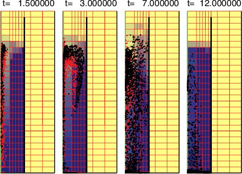
Figure 6. GPM10 (ZAO, subcool): comparison with experimental data on melt jet leading edge progress (a), water temperature (b), and containment pressure (c).

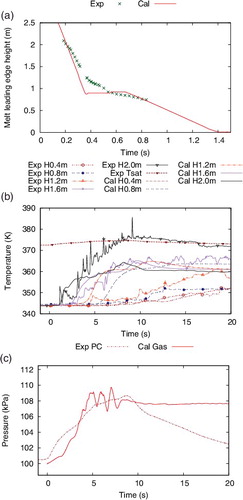
Figure 7. GPM10 (ZAO, subcool): sensitivity of model parameters on the re-agglomerate fraction (a) and heat transfer to water (b).

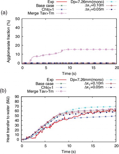
Figure 8. Snapshots of GPM05 (ZAO, shallow pool) simulation, base case (time 1.5, 3, 7, and 12 s) (red/black dots are molten/frozen particles).

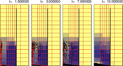
Figure 9. GPM05 (ZAO, shallow pool): sensitivity of model parameters on the re-agglomerate fraction (a) and heat transfer to water (b).

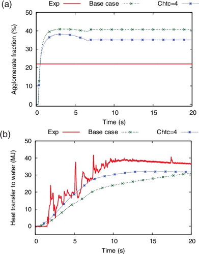
Figure 10. Snapshots of GPM12 (ZAO, saturation) simulation, C_htc = 4 (time 1.5, 3, 7, and 12 s) (red/black dots are molten/frozen particles).

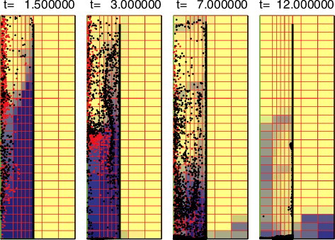
Figure 11. GPM12 (ZAO, saturation): sensitivity of model parameters on the re-agglomerate fraction (a) and heat transfer to water (b).

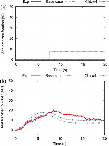
Figure 12. GPM09 (SUS, subcool): sensitivity of model parameters on the re-agglomerate fraction (a) and heat transfer to water (b).

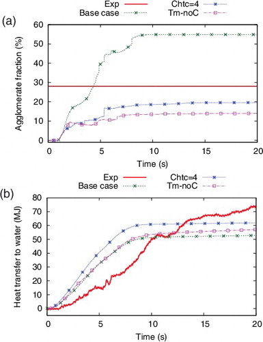
Figure 13. GPM08 (SUS, saturation): sensitivity of model parameters on the re-agglomerate fraction (a) and heat transfer to water (b).

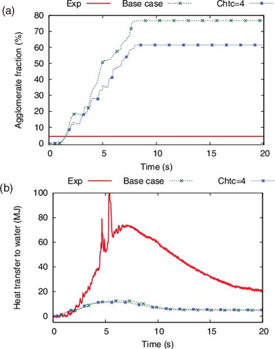
Figure 14. Comparison of the calculated containment pressure with experimental data for ALPHA/GPM. Calculation cases GPM10 and 05: base case, GPM12, 09, and 08: C_htc = 4.

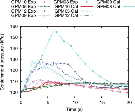
Figure 15. Comparison of calculated particle size distribution with experimental data for ALPHA/GPM. Calculation cases GPM10 and 05: base case, GPM12, 09, and 08: C_htc=4.

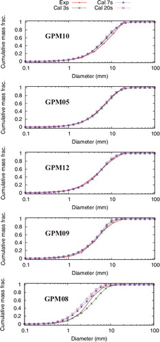
Figure 16. Analytical grid for FARO L14 (left) and L28/L31 (right) simulation.

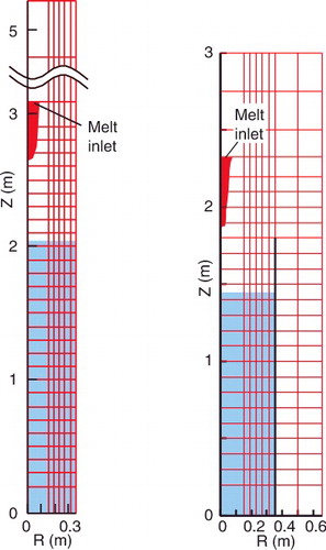
Table 4. Summary of conditions and results of selected FARO experiments [13].

FARO #	L14	L28	L31
Melt material, Mass (kg)	UO2–ZrO2^*1, 125	UO2–ZrO2, 175	UO2–ZrO2, 92
Melt T (K) (superheat)	3123 (283)	3052 (212)	2990 (150)
Melt release diameter (mm)	100	50	50
Melt free fall height (m)	1.04	0.89	0.77
System P (MPa)	5	0.5	0.2
Water T (K) (subcool)	537 (0)	424 (1)	291 (104)
Pool depth (m)	2.05	1.44	1.45
Jet breakup length (m)	–	0.9	0.83
Agglomerate fraction (%)	16	48	0
Debris MMD^*2 (mm)	4.8	3.0	3.4
Max. pressure (MPa)	7.8 (2.5 s)	1.67 (6.5 s)	0.26 (3 s)
Final pool T (K)	564	474	330

Note: ^*1UO₂–ZrO₂ 80:20 wt%; ^*2mass median diameter.

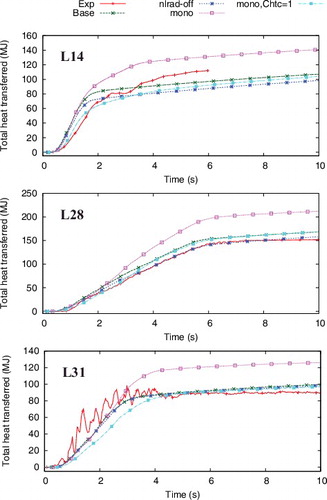
Figure 17. FARO L14, L28, and L31: comparison with experimental data on pressure (a), heat exchange (b), and agglomerate fraction (c).

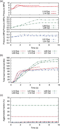
Figure 18. FARO L14, L28, and L31: comparison with experimental data on debris size distribution.

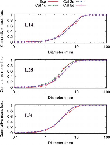
Figure 19. FARO L14, L28, and L31: impact of the modified models on the heat transfer: ‘nlrad-off’ non-local radiation model disabled, ‘mono’ mono-spectrum particle size at mass median diameter, ‘mono, C_htc = 1’ mono-spectrum particle size without heat transfer modification.

Moriyama K, Maruyama Y, Nakamura H. Steam explosion simulation code JASMINE v.3 user's guide. Tokai (Japan): Japan Atomic Energy Agency; 2008. (JAEA-Data/Code 2008-014).

 Google Scholar

Moriyama K, Maruyama Y, Usami T, et al. Coarse break-up of a stream of oxide and steel melt in a water pool. Tokai (Japan): Japan Atomic Energy Research Institute; 2005. (JAERI-Research 2005-017).

 Google Scholar

Annunziato A, Addabo C, Yerkess A, et al. FARO test L-14 on fuel-coolant interaction and quenching– comparison report. Volume I: analysis of the results – OECD/CSNI International standard problem 39. Paris (France): OECD/NEA/CSNI; 1998. (NEA/CSNI/R(97)31/Part I).

 Google Scholar

Kim CS. Thermophysical properties of stainless steels. Lemont (IL): Argonne National Laboratory; 1975. (ANL-75-55).

 Google Scholar

The Japan Society of Mechanical Engineers (JSME), editor. JSME data book: thermophysical properties of fluids. Tokyo (Japan): The Japan Society of Mechanical Engineers; 1994.

 Google Scholar

Magallon D. Characteristics of corium debris bed generated in large-scale fuel-coolant interaction experiments. Nucl Eng Des. 2006;236:1998–2009.

 Web of Science ®Google Scholar