Dead time corrections on the Feynman-Y curve using the backward extrapolation method

Figures & data

Figure 1. Paralyzing vs. non-paralyzing dead time. In the non-paralyzing model, the third detection (indicated by the black dot) is recorded, whereas in the paralyzing model it is not.

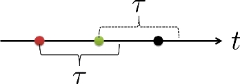
Figure 2. Inducing a paralyzing dead time on the detection signal. Each dot represents a detection. If the duration between two consecutive detections is less than the dead time, the later of the two is removed.

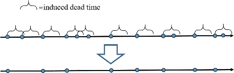
Figure 3. A three-dimensional plot of the BEX surface Y(T, τ). The black dots indicate the τ₀ cut-off, after which the induced dead time changes the values of the variance-to-mean ratio.

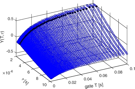
Figure 4. Graphic illustration of the BEX method on a single ‘slice’ of the Feynman-Y curve. The fitted curve is second-degree one-dimensional polynomial, i.e. p₀ + p₁τ + p₂τ².

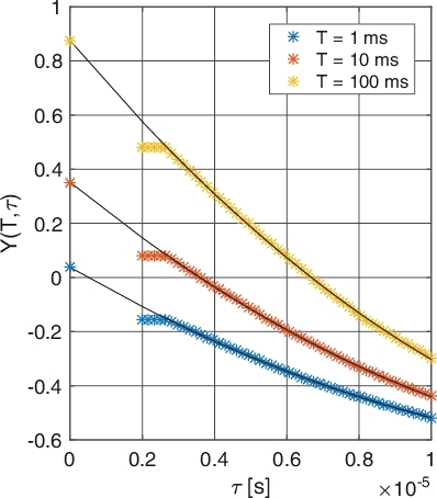
Figure 5. Graphic illustration of the BEX method on the entire Y(T, τ) surface (rather than a single value of T). The fitted surface is a fourth-degree two-dimensional polynomial, i.e. p₀₀ + p₁₀τ + p₀₁T + p₂₀τ² + p₁₁τT + p₀₂T² + p₃₀τ³ + p₂₁τ²T + p₁₂τT² + p₀₃T³ + p₄₀τ⁴ + p₃₁τ³T + p₂₂τ²T² + p₁₃τT³ + p₀₄T⁴.

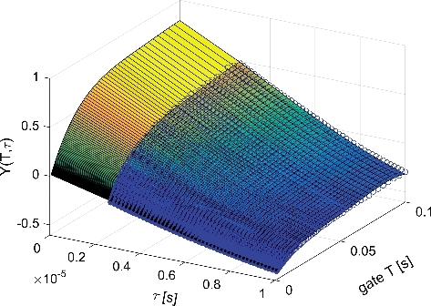
Figure 6. Schematic layout of the MINERVE zero power reactor during the noise measurements campaign in September 2014.

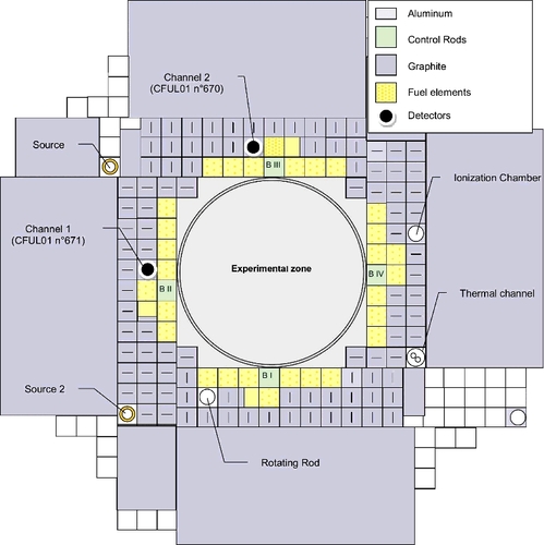
Table 1. Detector signals with inflicted dead time τ

Signal no.	Experiment	Detector	τ (µs)	CPS reduction
1	EXP1	1	1.37	5%
2			2.2	8%
3			2.7	10%
4		2	1.34	5%
5			2.15	8%
6			2.67	10%
7	EXP2	1	0.77	5%
8			1.2	8%
9			1.5	10%
10		2	0.72	5%
11			1.1	8%
12			1.4	10%

Figure 7. Results of the BEX method for all signals created from the first detector in EXP1.

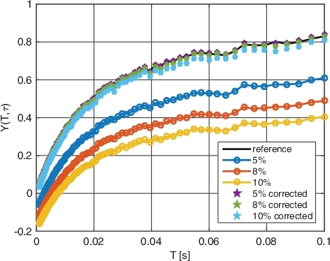
Figure 8. Results of the BEX method for all signals created from the second detector in EXP1.

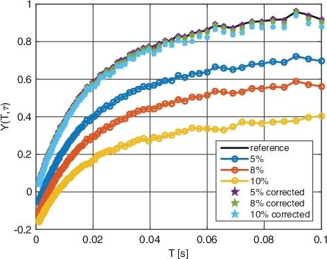
Figure 9. Results of the BEX method for all signals created from the first detector in EXP2.

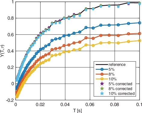
Figure 10. Results of the BEX method for all signals created from the second detector in EXP2.

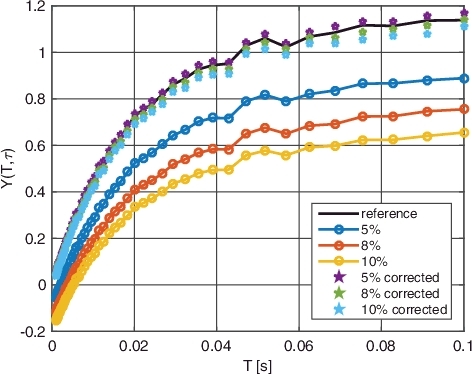
Table 2. Quantification of the goodness of the corrected curves (see Equation (7(7) $$\begin{array}{c}\hfill e_Y[\%]=\frac{1}{N}\sum _{k=1}^N\left|\frac{Y\left(T_k\right)-Y\left(T_k\right|\tau \to 0)}{Y\left(T_k\right)}\right|.\end{array}$$(7) )) for different induced dead times, i.e. 5%, 8%, and 10% CPS reduction (see Table 1)

CPS reduction		5%	8%	10%
EXP1	det. 1	1.5%	4.5%	10.7%
	det. 2	0.9%	2.1%	6.3%
EXP2	det. 1	3.8%	0.7%	3.2%
	det. 2	3.1%	3.8%	7.6%

Figure 11. The deviation (%) of the BEX approximation from the Feynman-Y curve with respect to the control values.

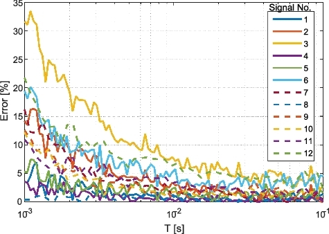
Table 3. The evaluated decay constant and reactivity using the BEX dead time correction method. The propagated uncertainty on the reactivity is approximately ±30 pcm

	α (s^-1)		ρ (pcm)
Signal no.	Estimated	Reference	Estimated	Reference
1	99.8	100.9	−208	−220
2	100.0	100.9	−210	−220
3	100.4	100.9	−214	−220
4	99.4	98.6	−204	−197
5	98.1	98.6	−192	−197
6	97.3	98.6	−185	−197
7	93.8	90.7	−152	−123
8	92.2	90.7	−137	−123
9	89.5	90.7	−112	−123
10	93.1	93.1	−146	−145
11	89.8	93.1	−115	−145
12	88.9	93.1	−107	−145