Demonstration of gamma-ray pipe-monitoring capabilities for real-time process monitoring safeguards applications in reprocessing facilities

Figures & data

Figure 1. The solution measurement and monitoring system provides continuous volumetric and density measurements of the solution in the tanks where the random verification samples are collected for isotopic composition evaluation. Present process inspection capabilities can be improved by monitoring gamma rays from solution flowing through pipes between tanks and process apparatuses.

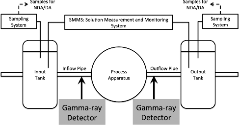
Figure 2. (a) A diagram of the shielded LaBr₃ detector measurement position in front of the transfer pipes relative to the sampling glovebox (GB) on the first floor (1F) and solution tanks in the basement (BF). The dashed arrows indicate the direction of the solution flow between the input tank and output tank. (b) A top-down view of the LaBr₃ shielded with high-density polyethylene (HDPE) and lead (Pb) in the horizontal position relative to the inflow and outflow transfer pipes. Shown vertically centered with the LaBr₃ axis, it can be seen that the GB struts attenuated the gamma rays (GRs) from each pipe differently due to their relative position with the detector.

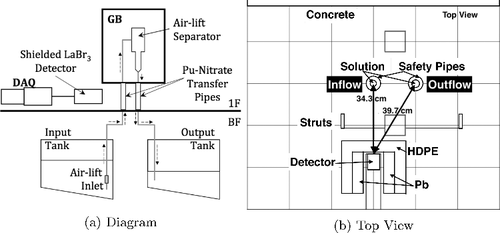
Figure 3. Screenshots from a movie showing a Pu-Nitrate surrogate solution moving through pipes similar to the PCDF equipment. Using the same type of pump system, bubbles can be seen intermixed with the solution in the pipes. Note that bubbles also exist in the outflow pipe and move upward toward the airlift separator. See online version for color.

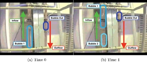
Table 1. Composition, density, and measurement days for the transferred Pu-Nitrate sample, P136, and a similar composition sample, P135

		P136	P135	Unit
Isotopic fractions	Pu-238	1.247	1.247	weight%
	Pu-239	56.989	56.966	weight%
	Pu-240	32.486	32.498	weight%
	Pu-241	3.175	3.182	weight%
	Pu-242	6.103	6.107	weight%
Pu concentration		136.6	160.9	g/L
Am-241 concentration		3.142	4.683	g/L
Density		1.373	1.411	g/cm^3
DA measurement day		6/6/2016	5/17/2016	m/d/y
Measurement day		6/14/2016	5/30/2016	m/d/y

Figure 4. (a) Change in volume of solution in the input tank (circles) and output tank (squares) during the transfer compared to the gamma-ray measurement at the glovebox pipe (gray line) in 1-s integration time bins relative to when the detector started collecting data. The missing electromanometer (EM) data points are due to temporarily stopping the automated computer for manual operation. (b) The beginning of the transferred solution gamma rays binned over 1-s and 100-ms integration periods. (c) The end of the transferred solution gamma rays binned over 1-s and 100-ms integration periods. In all images, the relevant times are indicated.

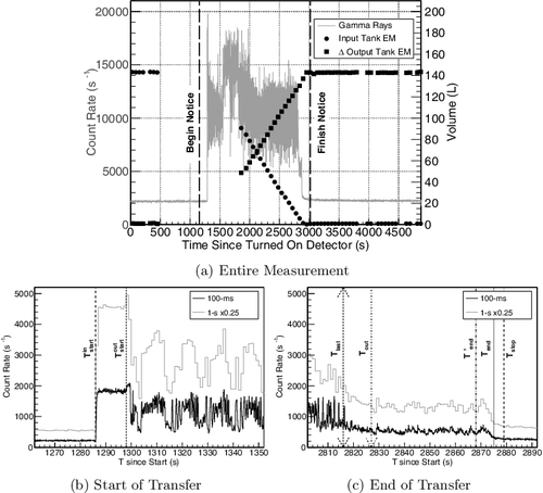
Table 2. The times that events occurred during the pipe-monitoring according to the lab notebook (Notes), the input tank (In) and output tank (Out) electromanometer (EM) data, and gamma-ray (GR) detector live-time. All times are in seconds referenced to the start of the detector data collection. The times with an asterisk (^*) are the values to be calculated in the process analysis (see Section 4.3)

	Label	Notes	EM	GR	Explanation
Beginning	^notesTb	1157	–	–	Notified transfer will begin
	^InTb	–	1249	^*	Solution begins flowing, input tank
	T^instart	–	–	1286	Solution first observed in inflow pipe
	T^outstart	–	–	1298	Solution first observed in outflow pipe
	^OutTb	–	1326	^*	Solution begins flowing, output tank
Ending	Tlast	–	-	2816	Solution finishes entering inflow pipe
	Tout	–	–	2827	Solution dominantly in outflow pipe
	T′end	–	–	2868	Last of solution enters outflow pipe
	Tend	–	–	2875	Last of solution leaves outflow pipe
	Tstop	–	–	2879	Return to hold-up plus activation rates
	^InTf	–	2884	^*	Solution finishes flowing, input tank
	^OutTf	–	2968	^*	Solution finishes flowing, output tank
	^notesTf	3017	–	–	Notified transfer finished

Figure 5. (a) The MCNP-modeled relative probability distribution (left) and cumulative distribution function (CDF) (right) of the vertical height from which gamma rays generated along the inflow pipe and outflow pipe (indicated in the legend) can be observed by the detector referenced from the top of the concrete floor. The horizontal lines indicate vertical positions as described in the text. (b) A simulation depicting the gamma-ray integrated count as a 5-cm length of the solution passes through the sensitive region of the inflow pipe, similar to Figure 3. The time (left) is calculated using the EM flow-rate converted into linear speed (see Section 4.1). The variable size of the circles in the position plot (right) indicates the relative intensity of the counts in the detector.

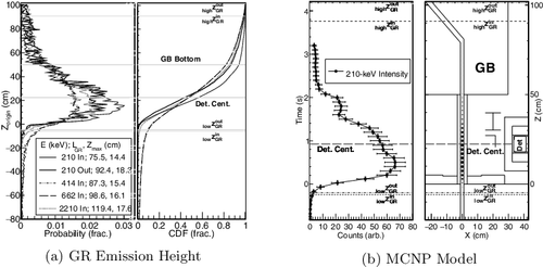
Figure 6. (a) An example of how I_A(t_i) (long dash) and I_B(t_i) (short dash) are determined from the data (solid) for a 1-s t_i time bin (filled gray). (b) The beginning of the transfer with 500-ms time bins clearly shows inflow solution pulsing following initial continuous flow before T^out_start. (c) The beginning of the transfer with 1-s integrations averages the inflow and outflow count-rates to produce aliased pulsing. The ϵ_F (dot-dash) indicates the trigger threshold level used to determine when there is a count-rate change.

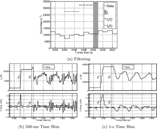
Figure 7. A comparison of the measured solution count rates per energy bin before (light gray), during (thick black), and after (dark gray) the transfer period in the 200- to 850-keV energy region. The P135 (dotted) spectrum measured statically with a HPGe in a different glovebox is arbitrarily scaled for comparison. The primary nuclide producing each gamma-ray peak is indicated for each prominent peak in the solution spectrum. The label ‘Ann.’ indicates the 511-keV annihilation peak.

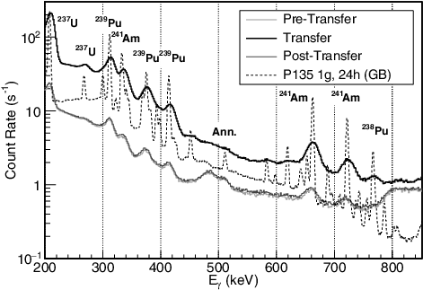
Figure 8. A comparison of the 1-s integrated count-rate over the entire measurement time for the integrated spectrum (total) and indicated gamma-ray peaks. The gamma rays appearing from the Pu-Nitrate sample all have a clear rise during the transfer time. The natural peak, derived from ⁴⁰K (1462 keV) and ¹³⁸La (1438 keV), is largely unaffected by the sample transfer. Also indicated is the average background rate of the 208-keV region (dotted line) from hold-up in the equipment, and the transfer beginning and finishing notice times (dashed lines).

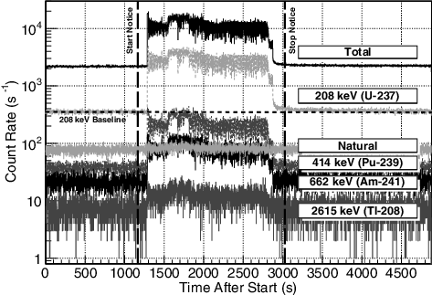
Table 3. The set of primary gamma-ray energy peaks observed during the transfer of Pu-Nitrate with the primary nuclide and calculated ratio R_γ for the period when solution is in the inflow pipe (see Table 2) for the three different pulsing possibilities defined for F (see Equation (3(3) $$\begin{array}{c}\hfill F\left(t_i\right)=ln\left(\frac{I_A\left(t_i\right)}{I_B\left(t_i\right)}\right),\end{array}$$(3) ) and Figure 6)

			Rγ = Nγ/N415 − keV
Emean	Primary	Erange	Mean (RMS)
(keV)	nuclide	[keV,keV]	Solution	Bubbles	${\bar{R}}_{\gamma }$
203	^237U	[190,220]	14.8 (8)	14.7 (8)	14.7 (8)
269	^237U	[255,285]	3.8 (2)	3.8 (2)	3.8 (2)
310	^239Pu	[295,325]	4.03 (20)	4.02 (19)	4.02 (19)
332	^241Am	[325,350]	2.5 (1)	2.4 (1)	2.4 (1)
373	^239Pu	[360,390]	1.67 (9)	1.67 (8)	1.67 (9)
415	^239Pu	[400,430]	1 (0)	1 (0)	1 (0)
658	^241Am	[635,680]	0.39 (4)	0.40 (4)	0.40 (4)
724	^241Am	[698,745]	0.25 (3)	0.26 (3)	0.25 (3)
767	^238Pu	[750,785]	0.14 (2)	0.14 (2)	0.14 (2)
1460	^40K/^138La	[1385,1525]	0.4 (1)	0.4 (1)	0.4 (1)
2208	^1H-act.	[2150,2270]	0.06 (2)	0.06 (2)	0.06 (2)
2609	^208Tl	[2530,2675]	0.05 (1)	0.05 (1)	0.05 (1)

Figure 9. Top: the 3-s integrated gamma-ray counts, N₆₅₈, between 635 and 680 keV (dominantly the ²⁴¹Am 662-keV gamma ray) for each time bin between the begin and finish notices. The gamma ray source types and event times noted in the legend are described in Section 2.2. ‘Other’ refers to no clear pulsing during the transfer and times outside of the transfer period. Bottom: the ratio, R₆₅₈, of the above gamma-ray peak counts compared to the peak counts dominated by the ²³⁹Pu 414-keV reference peak. While solution is in the inflow pipe, the ratio is within η₆₅₈ of the mean but increases when solution is only in the outflow pipe (T_last < t_i < T_end) before returning to the hold-up value. Relevant times are indicated.

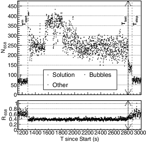
Figure 10. The 3-s integrated count spectra, C(t_i, E) (a), and the difference between consecutive spectra, S_i (b), at the beginning of the transfer for the times indicated in the legends for the same energy region shown in Figure 7. See online version for color.

Figure 11. The composition difference, S_i, average spectral deviation between consecutive time bins for the period shown in Figure 9. The variations are all caused by differences between the solution gamma-ray spectral distribution and the hold-up gamma-ray spectral distribution with the solution arrival producing a significant spike at 1287 s as shown in Figure 10. The error bars are the uncertainty of fitting S_i to a flat line. Relevant times are indicated.

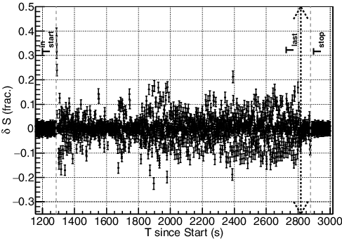
Table 4. Comparisons of values calculated from the gamma ray (GR) data and compared to the fits from the electromanometer (EM) data for the linear velocity (v_lin), volumetric flow-rates (R_V), and total volume transferred (V) through the inflow (in) and outflow (out) pipes. The inflow terms are calculated using the using Equations (13(13) $$\begin{array}{c}\hfill v_{lin}^{in}=\frac{L^{in}}{T_{start}^{out}-T_{start}^{in}-\frac{L^{out}}{v_{lin}^{out}}}\end{array}$$(13) ) and (14(14) $$\begin{array}{c}\hfill v_{lin}^{in}=\frac{L_{GB}{-}_{low}{z}_{GR}^{in}{-}_{high}{z}_{GR}^{out}}{T_{start}^{out}-T_{start}^{in}},\end{array}$$(14) ) as indicated. The v_lin and R_V are compared between the input (In) and output (Out) tank EM data calculated values (ΔX) with V compared to the average (bold). The values in parentheses are the uncertainty on the calculated last digit

Value	EM			GR	ΔX	Eq. #
vlin (cm/s)		In	24.2 (2)	27.0 (47)	2.8 (47)	(13(13) $$\begin{array}{c}\hfill v_{lin}^{in}=\frac{L^{in}}{T_{start}^{out}-T_{start}^{in}-\frac{L^{out}}{v_{lin}^{out}}}\end{array}$$(13) )
				26.7 (31)	2.5 (31)	(14(14) $$\begin{array}{c}\hfill v_{lin}^{in}=\frac{L_{GB}{-}_{low}{z}_{GR}^{in}{-}_{high}{z}_{GR}^{out}}{T_{start}^{out}-T_{start}^{in}},\end{array}$$(14) )
		Out	14.03 (9)	15.1 (17)	1.1 (17)	(7(7) $$\begin{array}{c}\hfill v_{lin}^{out}=\frac{L_{GR}^{out}}{\delta T_{end}}=\frac{{|}_{low}{z}_{GR}^{out}{-}_{high}{z}_{GR}^{out}|}{T_{end}-T_{end}^{\text{'}}},\end{array}$$(7) )
RV (mL/s)	86.6 (9)	In	87.0 (7)	97.1 (167)	10.1 (167)	(13(13) $$\begin{array}{c}\hfill v_{lin}^{in}=\frac{L^{in}}{T_{start}^{out}-T_{start}^{in}-\frac{L^{out}}{v_{lin}^{out}}}\end{array}$$(13) )
				96.0 (112)	9.0 (112)	(14(14) $$\begin{array}{c}\hfill v_{lin}^{in}=\frac{L_{GB}{-}_{low}{z}_{GR}^{in}{-}_{high}{z}_{GR}^{out}}{T_{start}^{out}-T_{start}^{in}},\end{array}$$(14) )
		Out	86.4 (5)	93.2 (103)	6.8 (103)	(7(7) $$\begin{array}{c}\hfill v_{lin}^{out}=\frac{L_{GR}^{out}}{\delta T_{end}}=\frac{{|}_{low}{z}_{GR}^{out}{-}_{high}{z}_{GR}^{out}|}{T_{end}-T_{end}^{\text{'}}},\end{array}$$(7) )
V (L)	141.7 (57)	In	142.2 (56)	148.5 (256)	6.3 (256)	(13(13) $$\begin{array}{c}\hfill v_{lin}^{in}=\frac{L^{in}}{T_{start}^{out}-T_{start}^{in}-\frac{L^{out}}{v_{lin}^{out}}}\end{array}$$(13) )
				146.8 (172)	4.6 (172)	(14(14) $$\begin{array}{c}\hfill v_{lin}^{in}=\frac{L_{GB}{-}_{low}{z}_{GR}^{in}{-}_{high}{z}_{GR}^{out}}{T_{start}^{out}-T_{start}^{in}},\end{array}$$(14) )
		Out	141.8 (10)	146.3 (162)	4.2 (162)	(7(7) $$\begin{array}{c}\hfill v_{lin}^{out}=\frac{L_{GR}^{out}}{\delta T_{end}}=\frac{{|}_{low}{z}_{GR}^{out}{-}_{high}{z}_{GR}^{out}|}{T_{end}-T_{end}^{\text{'}}},\end{array}$$(7) )

Table 5. Solution transfer begin (b) and finish (f) times calculated from the input (In) and output (Out) tank electromanometer (EM) data and gamma-ray (GR) data. The GR values were calculated from the solution linear speed, v_lin, shown in Table 4 for the pipe leading to the appropriate tank. The comparisons made between ^InT_b or ^OutT_f and the GR values (bold) define the true bounds of the transfer. All times are in seconds referenced to the start of the GR data collection. The values in parentheses are the uncertainty on the calculated last digit

Explanation	EM (s)		GR (s)	ΔT (s)	Eq. #
Solution flow begins	^InTb	1249 (39)	1257 (5)	8 (40)	(13(13) $$\begin{array}{c}\hfill v_{lin}^{in}=\frac{L^{in}}{T_{start}^{out}-T_{start}^{in}-\frac{L^{out}}{v_{lin}^{out}}}\end{array}$$(13) )
			1257 (2)	8 (39)	(14(14) $$\begin{array}{c}\hfill v_{lin}^{in}=\frac{L_{GB}{-}_{low}{z}_{GR}^{in}{-}_{high}{z}_{GR}^{out}}{T_{start}^{out}-T_{start}^{in}},\end{array}$$(14) )
	^OutTb	1326 (31)	1351 (7)	−28 (32)	(7(7) $$\begin{array}{c}\hfill v_{lin}^{out}=\frac{L_{GR}^{out}}{\delta T_{end}}=\frac{{|}_{low}{z}_{GR}^{out}{-}_{high}{z}_{GR}^{out}|}{T_{end}-T_{end}^{\text{'}}},\end{array}$$(7) )
Solution flow finishes	^InTf	2884 (39)	2846 (5)	−38 (40)	(13(13) $$\begin{array}{c}\hfill v_{lin}^{in}=\frac{L^{in}}{T_{start}^{out}-T_{start}^{in}-\frac{L^{out}}{v_{lin}^{out}}}\end{array}$$(13) )
			2846 (2)	−38 (39)	(14(14) $$\begin{array}{c}\hfill v_{lin}^{in}=\frac{L_{GB}{-}_{low}{z}_{GR}^{in}{-}_{high}{z}_{GR}^{out}}{T_{start}^{out}-T_{start}^{in}},\end{array}$$(14) )
	^OutTf	2968 (31)	2940 (7)	−28 (32)	(7(7) $$\begin{array}{c}\hfill v_{lin}^{out}=\frac{L_{GR}^{out}}{\delta T_{end}}=\frac{{|}_{low}{z}_{GR}^{out}{-}_{high}{z}_{GR}^{out}|}{T_{end}-T_{end}^{\text{'}}},\end{array}$$(7) )