Determination of humic substances in deep groundwater from sedimentary formations by the carbon concentration-based DAX-8 resin isolation technique

Figures & data

Table 1. Geological conditions at the Horonobe boreholes and the Niigata observation wells.

Sampling sites	Latitude (N, decimal)	Longitude (E, decimal)	Depth (GL – m)	Geological formation	Composition
Horonobe, Borehole 07-V140-M03	45.0456	141.8593	142.3–150.1	Koetoi F.	Diatomaceous mudstone
Horonobe, Borehole 08-E140-C01	45.0446	141.8602	157.6–167.9	Koetoi F.	Diatomaceous mudstone
Horonobe, Borehole 09-V250-M02	45.0453	141.8596	248.9	Transition*	Diatomaceous/siliceous mudstone
Horonobe, Borehole 10-E250-M01	45.0446	141.8601	247 – 248.8	Transition*	Diatomaceous/siliceous mudstone
Horonobe, Borehole 13-350-C01	45.0459	141.8596	348 – 349.4	Wakkanai F.	Siliceous mudstone
Horonobe, Borehole 14-350-C04	45.0452	141.8586	348.6–353.7	Wakkanai F.	Siliceous mudstone
Niigata, Observation well Nuttari-560 m	37.9196	139.0782	553.0–558.0**	Kanbara F.	Gravel, sand, mud
Niigata, Observation well Nishikambara-1050 m	37.8504	138.9804	972.0–1043.0**	Uonuma F.	Gravel, sand, mud

*Tradition zone between Koetoi and Wakkanai formations

**Screen depth

Figure 1. Sampling sites of the sedimentary groundwater.

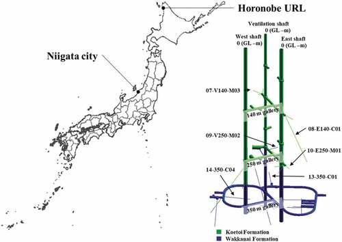
Table 2. Water qualities and concentrations of DOM and HS in the groundwater at the Horonobe boreholes and Niigata observation wells.

Sampling sites	Sampling date	Water type [34–36]	pH	EC (mS m^−1)	CDOM (mg-C dm^−3)	CHS (mg-C dm^−3)	%HS (%)
Horonobe, Borehole 07-V140-M03	Sep. 2016	Fossil seawater, Na-Cl (HCO3)*	7.4	1350	24.6 ± 0.6	15.9 ± 0.6	64.6 ± 1.7
Horonobe, Borehole 08-E140-C01	Sep. 2016	Fossil seawater, Na-Cl (HCO3)*	7.2	1240	20.0 ± 1.2	13.4 ± 1.6	67.0 ± 3.8
Horonobe, Borehole 09-V250-M02	Sep. 2016	Fossil seawater, Na-Cl (HCO3)*	7.3	860	12.5 ± 1.4	7.8 ± 0.4	62.8 ± 3.8
Horonobe, Borehole 10-E250-M01	Sep. 2016	Fossil seawater, Na-Cl (HCO3)*	7.3	800	15.3 ± 1.0	10.2 ± 1.3	66.3 ± 4.3
Horonobe, Borehole 13-350-C01	Sep. 2016	Fossil seawater, Na-Cl (HCO3)*	7.4	1990	17.3 ± 0.2	10.6 ± 0.4	60.9 ± 2.0
Horonobe, Borehole 14-350-C04	Sep. 2016	Fossil seawater, Na-Cl (HCO3)*	7.0	1660	20.7 ± 0.7	12.6 ± 0.6	61.1 ± 1.3
Niigata, Observation well Nuttari-560 m	Aug. 2017	Fossil seawater, Na-Cl	7.4	1970	19.3 ± 0.3	12.3 ± 0.1	63.6 ± 0.4
Niigata, Observation well Nishikambara-1050 m	Feb. 2017	Fossil seawater, Na-Cl	7.3	3540	40.5 ± 1.0	23.5 ± 1.1	58.0 ± 4.2

* HCO₃ is a measurable component [34]

Figure 2. Relationships between the HS proportion (%HS) and the dilution factor (f_d) in the different groundwater samples.

Figure 3. Relationships between C_DOM and C_HS in the groundwater at the Horonobe boreholes and Niigata observation wells and the result of the linear regression analysis.

Figure 4. Comparisons between the %HS measured by the carbon concentration-based DAX-8 resin isolation technique and the constant %HS defined as the slope of the regression analysis. The constant %HS from the literatures was calculated by the linear regression analysis as an intercept of zero. $\mathrm{R}\mathrm{M}\mathrm{S}\mathrm{E}=\sqrt{\frac{1}{n}\sum _i{\left(y_{\mathrm{o}\mathrm{b}\mathrm{s},\mathrm{i}}-y_{\mathrm{p}\mathrm{r}\mathrm{e}\mathrm{d},\mathrm{i}}\right)}^2}$, where n is a number of sample. y_obs,i and y_pred,i arethe experimentally determined and predicted %HS (i.e. the slope of the linear regression), respectively.

Miyakawa K, Mezawa T, Mochizuki A, et al. Data of groundwater chemistry obtained in the Horonobe underground research laboratory project (FY2014–2016). Horonobe: JAEA; 2017. (JAEA-Data/Code 2017–012).

 Google Scholar

Advanced Industrial Science and Technology (AIST), Japan Atomic Energy Agency (JAEA), Radioactive Waste Management Funding and Research Center (RWMC), et al. A commission investigation of geological disposal technology: development of enhancing the disposal system in the coastal region. Tokyo: METI; 2018. Japanese.

 Google Scholar