Modeling of gap conductance for LWR fuel rods applied in the BISON code

Figures & data

Table 1. Brief summary of the models that are available in BISON.

Default	New feature
Fill gas thermal conductivity models
Based on MATPRO-11 [13]	Pressure-effects are included to the code [20].
$\lambda ($W/m-K$)=a{T}^b$	$\lambda ($W/m-K$)={\lambda }^0(T)+{\lambda }_c^{\star }{\mathrm{\Psi }}_k\left(\frac{\rho }{{\rho }_c}\right)$
where	where
$T=$ temperature (K)	$\lambda =$ thermal conductivity of pure dilute gas (W/m-K)
$a,b=$ empirical coefficients vary for each gas	${\lambda }_c^{\star }=$ pseudo-critical thermal conductivity (W/m-K)
	${\mathrm{\Psi }}_k\left(\rho /{\rho }_c\right)$= the excessive thermal conductivity
	$\rho$= gas density (see Appendix A)
Temperature jump distance models
Kennard’s model based on a review by [14]	Kennard’s model based on a review by [12]
$g($cm$)=2878\left(\frac{2-\alpha }{\alpha }\right)\left(\frac{\lambda \sqrt{T}}{P}\right){\left(\frac{1}{{\sum }_{i=1}^n{f}_i/M_i}\right)}^{1/2}$	$g$(m)$=\frac{\sqrt{8\pi }}{(1+\gamma )\nu }\frac{\lambda }{P{\mathrm{\Lambda }}_{12}}\sqrt{\frac{T}{R_{g}M}}$
where	where
$T=$ temperature (K)	$T=$ temperature (K)
$P=$ pressure (dyne/cm${ }^2$)	$P=$ pressure (Pa)
$\lambda =$ fill gas thermal conductivity (cal/sec-cm-${ }^{\circ }$C)	$\lambda =$ fill gas thermal conductivity (W/m-K)
$M=$ molecular weight of gas constituent (g/mole)	$M=$ molecular weight of gas constituent (g/mole)
$f=$ mole fraction	$R_g=$ ideal gas constant (8.314 J/mol-K)
$\alpha =$ thermal accommodation coefficient	$\alpha =$ thermal accommodation coefficient
	$\frac{\sqrt{8\pi /R_g}}{(1+\gamma )\nu }=\left\{\begin{array}{cc}0.2173& \mathrm{f}\mathrm{o}\mathrm{r}\mathrm{t}\mathrm{h}\mathrm{e}\mathrm{m}\mathrm{o}\mathrm{n}\mathrm{a}\mathrm{t}\mathrm{o}\mathrm{m}\mathrm{i}\mathrm{c}\mathrm{g}\mathrm{a}\mathrm{s}\mathrm{e}\mathrm{s},\\ 0.1149& \mathrm{f}\mathrm{o}\mathrm{r}\mathrm{t}\mathrm{h}\mathrm{e}\mathrm{d}\mathrm{i}\mathrm{a}\mathrm{t}\mathrm{o}\mathrm{m}\mathrm{i}\mathrm{c}\mathrm{g}\mathrm{a}\mathrm{s}\mathrm{e}\mathrm{s},\\ 0.1242& \mathrm{f}\mathrm{o}\mathrm{r}\mathrm{t}\mathrm{h}\mathrm{e}\mathrm{p}\mathrm{o}\mathrm{l}\mathrm{y}\mathrm{a}\mathrm{t}\mathrm{o}\mathrm{m}\mathrm{i}\mathrm{c}\mathrm{g}\mathrm{a}\mathrm{s}\mathrm{e}\mathrm{s}.\end{array}\right.$
	${\mathrm{\Lambda }}_{12}=\left\{\begin{array}{cc}\frac{\alpha }{2-\alpha }& \mathrm{p}\mathrm{l}\mathrm{a}\mathrm{n}\mathrm{e},\\ \frac{\alpha }{1+(1-\alpha )r_1/r_2}& \mathrm{c}\mathrm{y}\mathrm{l}\mathrm{i}\mathrm{n}\mathrm{d}\mathrm{e}\mathrm{r},\\ \frac{\alpha }{1+(1-\alpha )(r_1/r_2{)}^2}& \mathrm{s}\mathrm{p}\mathrm{h}\mathrm{e}\mathrm{r}\mathrm{e}.\end{array}\right.$
Thermal accommodation coefficient models
based on a review by [14]	Toptan’s model [12]
$\alpha ={\alpha }_{He}+\frac{({\alpha }_{Xe}-{\alpha }_{He})(M_{mix}-M_{He})}{(M_{Xe}-M_{He})}$	$\alpha =1-\left(1-{\alpha }_{\mathrm{\infty }}tanh\left[\frac{\sqrt{m_{i}T}}{{\alpha }_{\mathrm{\infty }}}{\theta }_1\right]\right)exp\left(-\frac{{\theta }_2}{T}\right)$
where	where
${\alpha }_{He}=0.423-2.3\times {10}^{-4}T$	$T=$ temperature (K)
${\alpha }_{Xe}=0.749-2.5\times {10}^{-4}T$	${\alpha }_{\mathrm{\infty }}=2.4\mu /(1+\mu {)}^2$
$T=$ temperature (${ }^{\circ }$C)	$\mu =(M_i/M_s)$, the ratio of molecular weights
	$\theta =\{{\theta }_1,{\theta }_2\}$= the coefficient matrix
Meyer’s hardness models
an average value by [15]	MATPRO model [13]
$H$(N/m${ }^2)=$0.68 $\times {10}^9$	$H$(N/m${ }^2)=exp(26.034-2.6394\times {10}^{-2}T+4.35\times {10}^{-5}$$T^2+2.5621\times {10}^{-8}{T}^3)$
	where
	$T=$ temperature (K)

Figure 1. Sobol’ indices of six input parameters for a variety of inert gases in the open gap configuration with a (a) non-zero and (b) zero temperature jump distance. The larger the sensitivity indices, the more critical the parameters are for $h_{gap}$.

Figure 2. Sobol’ indices of six input parameters for a variety of inert gases in the open gap configuration with a (a) non-zero and (b) zero temperature jump distance. The larger the sensitivity indices, the more critical the parameters are for $h_{gap}$.

Figure 3. Sobol’ indices of eight input parameters for a variety of inert gases in the closed gap configuration. The larger the sensitivity indices, the more critical the parameters are for $h_{gap}$.

Table 2. Problem setup for the sensitivity analysis for both open and closed gap configurations. Three representative cases are considered to study the effects of input parameters on the gap conductance (1) for a larger gap thickness as compared to the sum of surface roughnesses in the open gap; (2) for a gap thickness which is in the order of the sum of surface roughnesses in the open gap, which is also representative for a closed gap with negligible load-to-hardness ratio; and (3) for a non-zero gap thickness with a non-negligible load-to-hardness ratio in the closed gap.

No.			$d$	$T$	$P$	${\epsilon }_{f,c}$	${\theta }_1$	${\theta }_2$	$(W/H)$
1	initial${ }^{\star }$	open gap (Figure 1)	10.0$\mu$m	600 K	1.0MPa	0.5$\mu$m	0.605	10.0	0.0
2		open gap (Figure 2)	1.0$\mu$m		5.0MPa
3		closed gap (Figure 3)							1.0
perturbation over the range:			[0.5,1.5]	[0.5,1.5]	[0.5,1.5]	[0.5,1.5]	[0.5,1.5]	[0.5,1.5]	[0.0,1.0]

Table 3. Overview of the fuel centerline temperature experimental data for BISON integral effects validation.

Experiment	Rod	Final Bu. (MWd/kgU)	FCT	FGR	Refs.
IFA431	1	$\approx 4$	✓		[17]
	2	$\approx 4$	✓		[17]
	3	$\approx 4$	✓		[17]
IFA432	1	$\approx 32$	✓		[17,18]
	2	$\approx 32$	✓		[17,18]
	3	$\approx 32$	✓		[17,18]
IFA515.10	A1	86.6	✓		[22]
IFA562.2	15	56.7	✓	✓	[23]
	16	56.2	✓	✓	[23]
	17	56.2	✓	✓	[23]
Risø-3	AN3	42.0	✓	✓	[18]
	AN4	42.0	✓	✓	[18]

IFA, instrumented fuel assembly

FCT, fuel centerline temperature

FGR, fission gas release.

Figure 4. BOL measured vs. predicted fuel centerline temperature for fuel rods in IFA-431, IFA-432, and IFA-515.10 using (a) Equation (2)(2) $h_{gap}=\frac{{\lambda }_g}{d+{\theta }_1({\xi }_1+{\xi }_2)+(g_1+g_2)}+\frac{{\theta }_2\mathrm{\Lambda }}{\sqrt{{\xi }_1+{\xi }_2}}\left(\frac{W}{H}\right),$(2) with the default modeling options in Table 1, denoted by PRIOR and (b) Equation (5)(5) $\begin{array}{cc}{h}_{gap}& =\frac{{\lambda }_g}{d+0.605({\xi }_1+{\xi }_2)+(g_1+g_2)}+\frac{10\mathrm{\Lambda }}{\sqrt[4]{0.5({\xi }_1^2+{\xi }_2^2)}}\left(\frac{W}{H}\right),\\ \theta & =\{{\theta }_1,{\theta }_2\}=\left\{0.605,\frac{10.0}{\sqrt[4]{0.5}}\right\}\end{array}$(5) with the new modeling options in Table 1, denoted by PRESENT (LTC = lower thermocouple measurement; UTC = upper thermocouple measurement; M = measured; P = predicted).

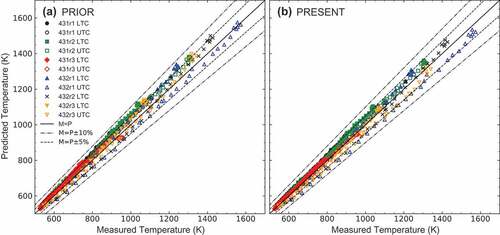
Table 4. The BOL validation metrics for the fuel centerline temperature predictions (Figure 4).

	$d$(K)	$d_M$(K)	$R_2$(–)	RMSE(K)	rRMSE(%)
prior	777.3	14,248.7	0.981	35.3	3.7
present	629.3	10,850.5	0.986	28.6	3.0

Figure 5. The average linear heat rate histories for (a) the Halden IFA-515.10 irradiation and (b) the Halden IFA-562 irradiation.

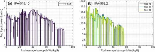
Figure 6. Measured fuel centerline temperatures against the BISON predictions for IFA-515.10 Rod A1, IFA-562.2 Rod 15, IFA-562.2 Rod 16, and IFA-562.2 Rod 17 at four different burnup ranges using (a) Equation (2)(2) $h_{gap}=\frac{{\lambda }_g}{d+{\theta }_1({\xi }_1+{\xi }_2)+(g_1+g_2)}+\frac{{\theta }_2\mathrm{\Lambda }}{\sqrt{{\xi }_1+{\xi }_2}}\left(\frac{W}{H}\right),$(2) with the default modeling options in Table 1 (PRIOR) and (b) Equation (5)(5) $\begin{array}{cc}{h}_{gap}& =\frac{{\lambda }_g}{d+0.605({\xi }_1+{\xi }_2)+(g_1+g_2)}+\frac{10\mathrm{\Lambda }}{\sqrt[4]{0.5({\xi }_1^2+{\xi }_2^2)}}\left(\frac{W}{H}\right),\\ \theta & =\{{\theta }_1,{\theta }_2\}=\left\{0.605,\frac{10.0}{\sqrt[4]{0.5}}\right\}\end{array}$(5) with the new modeling options in Table 1 (PRESENT). The selected rods are irradiated to high burnups; 75.5GWd/t UO${ }_2$ for IFA-515.10 Rod A1 and approximately 49.4GWd/t UO${ }_2$ for IFA-562.2 rods (M = measured; P = predicted). Four different burnup ranges are considered: (1) 0$\le$Bu$<$20, (2) 20$\le$Bu$<$40, (3) 40$\le$Bu$<$60, and (4) Bu$\ge$60 GWd/t UO${ }_2$.

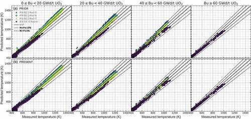
Table 5. The through-life validation metrics for the fuel centerline temperature predictions (Figure 6).

	PRIOR†				PRESENT‡
	R^2	ΔTmax	RMSE	rRMSE	R^2	ΔTmax	RMSE	rRMSE
	(—)	(K)	(K)	(%)	(—)	(K)	(K)	(%)
	IFA-562.2 Rod 15
0≤Bu<20	0.814	126.6	84.2	7.5	0.990	49.1	25.6	2.4
0≤Bu<20	0.830	139.8	90.3	8.6	0.980	69.4	33.9	3.2
40≤Bu<60	0.933	112.1	62.0	6.7	0.988	57.3	24.3	2.7
Overall	0.868	130.6	83.8	7.8	0.988	59.6	28.7	2.7
	IFA-562.2 Rod 16
0≤Bu<20	0.861	113.6	74.7	6.5	0.997	34.2	14.4	1.5
0≤Bu<20	0.917	90.6	57.2	5.3	0.998	35.3	10.7	1.2
40≤Bu<60	0.969	74.7	40.9	4.4	0.997	30.8	11.5	1.4
Overall	0.927	104.1	63.3	5.8	0.997	38.9	13.9	1.5
	IFA-562.2 Rod 17
0≤Bu<20	0.931	94.2	58.9	5.1	0.997	18.0	14.1	1.5
20≤Bu<40	0.964	79.1	44.4	4.2	0.997	28.7	13.7	1.5
40≤Bu<60	0.972	69.6	38.1	4.1	0.998	26.9	10.1	1.3
Overall	0.963	87.5	49.9	4.6	0.997	26.9	14.0	1.6
	IFA-515.10 Rod A1
0≤Bu<20	0.968	48.0	28.9	4.6	0.937	50.6	38.6	5.7
20≤Bu<40	0.976	54.0	27.1	4.8	0.939	60.1	37.5	6.1
40≤Bu<60	0.963	98.1	33.1	8.3	0.964	98.1	32.5	8.1
Bu≥60	0.981	69.1	24.1	5.2	0.982	69.1	23.5	5.2
Overall	0.972	63.9	28.6	5.3	0.953	66.6	34.7	6.0

†Equation (2)(2) $h_{gap}=\frac{{\lambda }_g}{d+{\theta }_1({\xi }_1+{\xi }_2)+(g_1+g_2)}+\frac{{\theta }_2\mathrm{\Lambda }}{\sqrt{{\xi }_1+{\xi }_2}}\left(\frac{W}{H}\right),$(2) with the default modeling options;

‡Equation (5)(5) $\begin{array}{cc}{h}_{gap}& =\frac{{\lambda }_g}{d+0.605({\xi }_1+{\xi }_2)+(g_1+g_2)}+\frac{10\mathrm{\Lambda }}{\sqrt[4]{0.5({\xi }_1^2+{\xi }_2^2)}}\left(\frac{W}{H}\right),\\ \theta & =\{{\theta }_1,{\theta }_2\}=\left\{0.605,\frac{10.0}{\sqrt[4]{0.5}}\right\}\end{array}$(5) with the new modeling options.

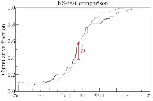
Figure 7. KS-test comparison: cumulative fraction plot of the fuel centerline temperature predictions for IFA-515 Rod A1 and IFA-562.2 Rod 15/16/17. The KS statistics are provided on the plot; KS statistic, $D$ – the largest vertical difference between the CDFs of the two samples – and $p$-value. Note that the value of the KS test statistics are not affected by scale changes such as using a log-scale as the test is robust and takes into account only the relative distribution of the data.

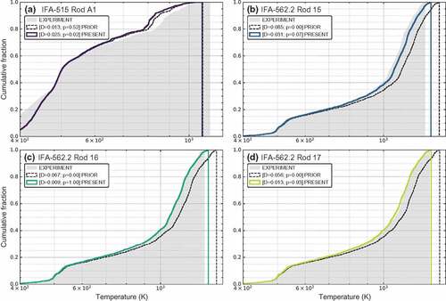
Figure 8. The BISON predictions vs. Risø-3 AN3 measurements for (a) fuel centerline temperature, and (b) fission gas release using the ‘prior’ and ‘present’ options (Grey shaded areas represent a $\pm$5% change around the experimental data.). At EOL, the predicted fission gas release is 26.8% with the ‘prior’ option and 21.0% with the ‘present’ option. Meanwhile, the measured value is 38.3%.

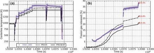
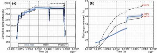
Figure 9. The BISON predictions vs. Risø-3 AN4 measurements for (a) fuel centerline temperature, and (b) fission gas release using the ‘prior’ and ‘present’ options (Grey shaded areas represent a $\pm$5% change around the experimental data.). At EOL, the predicted fission gas release is 54.4% with the ‘prior’ option and 39.7% with the ‘present’ option. Meanwhile, the measured value is 43.0%.

Table

Algorithm 1 Algorithm to find the largest real root of the cubic equation to assign the gas density analytically.

1: procedure

2:     define $\pi =4.0arctan(1.0)$,

3:     initialize $Re=\{0.0\}$ and $Im=\{0.0\}$,

4:     compute $p=\frac{(b^2-3ac)}{9a^2}$; $q=\frac{(9abc-27a^{2}d-2b^3)}{54a^3}$; and $\mathrm{o}\mathrm{f}\mathrm{f}\mathrm{s}\mathrm{e}\mathrm{t}=b/3a$,

5:     compute the discriminant, $\mathrm{\Delta }=(p^3-q^2)$,

6:     if $\mathrm{\Delta }>0$ then

7:        compute $\theta =arccos(q/p\sqrt{p})$ and $r=2\sqrt{p}$

8:        for $n=1,2,3$ do

9:          $Re[n]=r\ast cos\left(\frac{\theta +2(n-1)\pi }{3.0}\right)-\mathrm{o}\mathrm{f}\mathrm{f}\mathrm{s}\mathrm{e}\mathrm{t}$

10:          $Im[n]=0.0$

11:     else

12:        compute ${\gamma }_{1,2}=(q\pm \sqrt{-\mathrm{\Delta }}{)}^{1/3}$

13:        $Re[1]=({\gamma }_1+{\gamma }_2)-\mathrm{o}\mathrm{f}\mathrm{f}\mathrm{s}\mathrm{e}\mathrm{t}$

14:        $Re[2]=Re[3]=-\frac{1}{2}({\gamma }_1+{\gamma }_2)-\mathrm{o}\mathrm{f}\mathrm{f}\mathrm{s}\mathrm{e}\mathrm{t}$

15:        if $\mathrm{\Delta }\ne 0$ then

16:          calculate the complex conjugate roots

17:          $Im[2]=({\gamma }_1+{\gamma }_2)\sqrt{3}2$

18:          $Im[3]=-({\gamma }_1+{\gamma }_2)\sqrt{3}2$

19:     initialize $maxRealRoot=0.0$

20:     for n=1,2,3 do

21:        find the maximum real value

22:        if maxRealRoot $\le Re[n]$ and $Im[n]=0.0$ then

23:          maxRealRoot= $Re[n]$

Table 6. Comparison of the largest real value that is indicated by the bold numerical value. The cubic equation is given by $a{x}^3+b{x}^2+cx+d=0$.

$\{a,b,c,d\}$	Hard-coded in C++	Python	Cubic Eq’n Solver [30]
$\{1,3,3,1\}$	−1.00000	−1.00000 + 5.68937e-6$\cdot$j	−1.0000
		−1.00000–5.68937e-6$\cdot$j
		−1.00001
$\{1,-3,3,-1\}$	1.00000	1.00000 + 5.69146e-6$\cdot$j	1.0000
		1.00000–5.69146e-6$\cdot$j
		1.00001
$\{2,3,-8,3\}$	−3.00000	−3.00000	−3.0000
	0.50000	0.50000	0.5000
	1.00000	1.00000	1.0000
$\{1,5,5,-28\}$	−3.35223 + 2.27817$\cdot$j	−3.35223 + 2.27817$\cdot$j	−3.3522 + 2.2782$\cdot$j
	−3.35223–2.27817$\cdot$j	−3.35223–2.27817$\cdot$j	−3.3522–2.2782$\cdot$j
	1.70446	1.70446	1.7045

Figure 10. Schematic illustration of the Kolmogorov–Smirnov statistic (i.e., the largest vertical difference between the CDFs of the two samples). Note that $p$-value indicates the statistical significance between the two samples.

Hagrman DL, Reymann GA, Manson RE. MATPRO-version 11 (rev. 1): a handbook of materials properties for use in the analysis of light water reactor fuel rod behavior. Idaho Falls (ID): Idaho National Engineering Laboratory; 1980. NUREG/CR-0497, TREE-1290. doi:10.2172/6442256.

 Google Scholar

Toptan A, Kropaczek D, Avramova M. On the validity of the dilute gas assumption for gap conductance calculations in nuclear fuel performance codes. Nucl Eng Des. 2019;350:1–8.

 Web of Science ®Google Scholar

Lanning DD, Hann CR. Review of review of methods applicable to the calculation of gap conductance in Zircaloy-Clad UO₂ fuel rods. USA: Pacific Northwest Laboratory; 1975. BNWL-1894. doi:10.2172/4209005.

 Google Scholar

Toptan A, Kropaczek D, Avramova M. Gap conductance modeling I: theoretical considerations for single- and multi-component gases in curvilinear coordinates. Nucl Eng Des. 2019;353:110283.

 Web of Science ®Google Scholar

Jacobs G, Todreas N. Thermal contact conductance in reactor fuel elements. Nucl Sci Eng. 1973;50(3):283–306.

 Web of Science ®Google Scholar

Hann C, Lanning D, Bradley E, et al. Data report for the NRC/PNL Halden assembly IFA-432. PNL, 1978, NUREG/CR-0560; PNL-2673. doi:10.2172/6401826.

 Google Scholar

Sartori E, Killeen J, Turnbull J International fuel performance experiments (IFPE) database. OECD-NEA, 2010. [Accessed September 2019] Available at www.oecd-nea.org/science/fuel/ifpelst.html.

 Google Scholar

Tverberg T, Amaya M. Study of thermal behaviour of UO₂ and (U,Gd)O₂ to high burnup (IFA-515). Norway: OECD Halden Reactor Project; 2001. ( HWR-671).

 Google Scholar

Lösönen P. Early-in-life Irradiation of IFA-562.2 (the ultra high burn-up experiment). Norway: OECD Halden Reactor Project; 1989. ( HWR-247).

 Google Scholar

Wolfram—alpha widgets: cubic equation solver. [ Online; cited 2019 Dec 5]. Available at https://www.wolframalpha.com/widgets/view.jsp?id=1beb192fcbfba3b6afa17b00ae68605a

 Google Scholar