Development of local-scale high-resolution atmospheric dispersion model using large-eddy simulation part 6: introduction of detailed dose calculation method

Figures & data

Figure 1. Response function of ⁸⁵Kr from a source region to the surroundings based on prior PHITS simulations

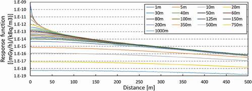
Figure 2. Schematic of the calculation of the dose rate distributions: (a) target area for estimating dose rate distribution; (b) target cell established in area (A); (c) region considering the dose contribution to the target cell (B); (d) LOHDIM-LES calculation area [15]

Figure 3. Schematic of the calculation of the dose rate distributions considering building shielding effects. (b) and (c) are the same as those in Figure 2

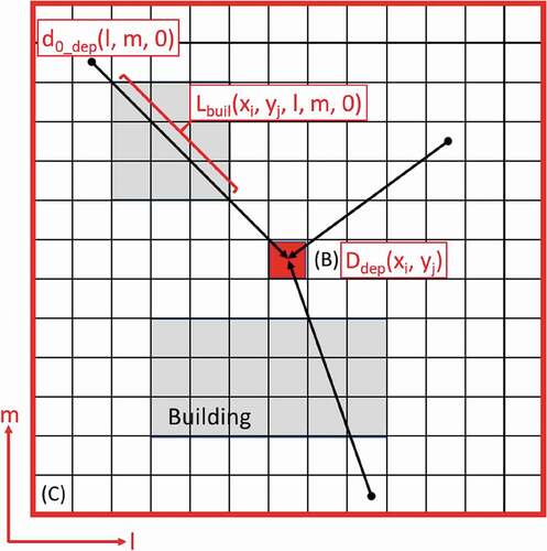
Figure 4. Calculation flow of LOHDIM-LES integrated with the dose calculation module SIBYL, which can be run with a postprocessing option

Figure 5. Spatial distributions of the air dose rates of ¹³⁷Cs produced by (a) the plume and (b) surface deposition at a height of 1 m. The circle indicates the point source location

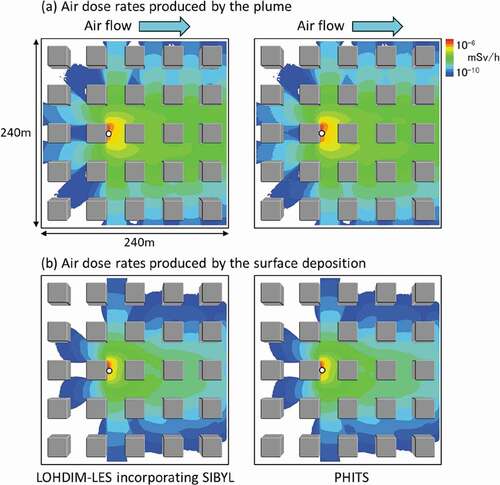
Figure 6. Study site in the nuclear fuel reprocessing plant in Rokkasho. The photograph on the left is reproduced by Google Earth graphics. The figure on the right shows the computational area of the study site. The square, star, and circle depict the plume stack, meteorological observation station, and MPs, respectively

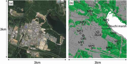
Figure 7. Time series of atmospheric stability during the two simulation periods (cases 1 and 2). The characters A-F indicate the atmospheric stability classes

Figure 8. Computational model

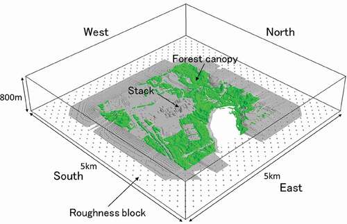
Figure 9. Time series of the ⁸⁵Kr release rate for the two simulation periods

Figure 10. Time series of the plume rise estimated by the optimized CONCAWE formulation for the two simulation periods

Figure 11. Time series of the wind speeds and directions at the stack height during the simulation period from 0900 JST to 1900 JST on 17 June 2008

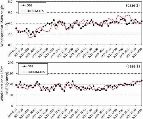
Figure 12. Time series of the wind speeds and directions at the stack height during the simulation period from 0600 JST to 1130 JST 18 June 2008

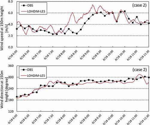
Figure 13. Instantaneous plume dispersion fields at 730 JST on 17 June 2008 (case 1) and 1040 JST on 18 June 2008 (case 2)

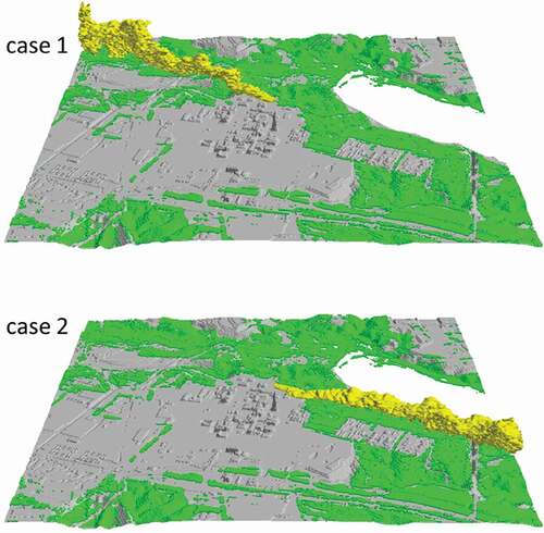
Figure 14. Time series of the 10-minute mean air concentrations of ⁸⁵Kr at each MP from 0900 JST to 1900 JST on 17 June 2008

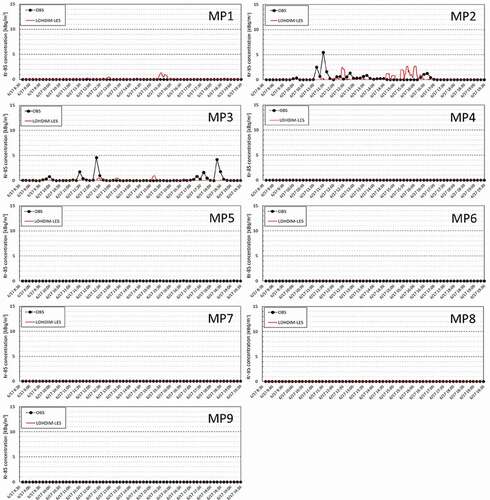
Figure 15. Time series of the 10-minute mean air concentrations of ⁸⁵Kr at each MP from 0600 JST to 1130 JST on 18 June 2008

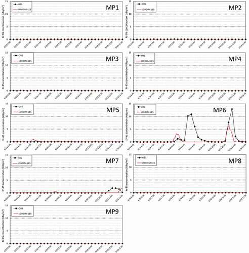
Figure 16. Time series of the air dose rate at each MP from 0900 JST to 1900 JST on 17 June 2008

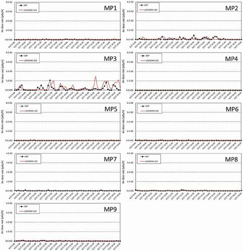
Figure 17. Time series of the air dose rate at each MP from 0600 JST to 1130 JST on 18 June 2008

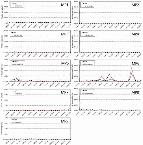
Figure 18. Scatter plot of the air dose rate. The solid and dashed lines indicate the perfect and FAC2 lines, respectively

Satoh D, Nakayama H, Furuta T, et al. Simulation code for estimating external gamma-ray doses from a radioactive plume and contaminated ground using a local-scale atmospheric dispersion model. Plos One. 2021. DOI:https://doi.org/10.1371/journal.pone.0245932.g011

 Web of Science ®Google Scholar