Quantitative visualization of a radioactive plume with harmonizing gamma-ray imaging spectrometry and real-time atmospheric dispersion simulation based on 3D wind observation

Figures & data

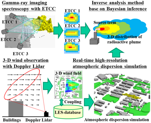
Figure 1. Proposed monitoring method for the quantitative visualization of a radioactive plume.

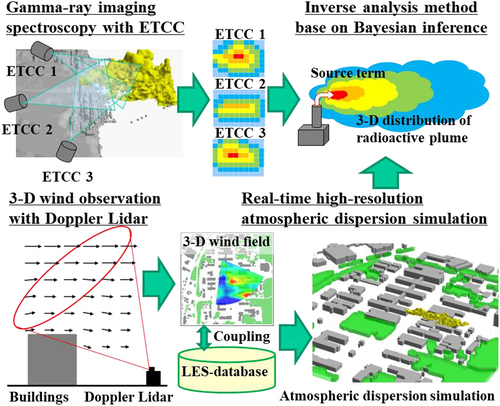
Figure 2. Schematic view of ETCC and schematic explanation of difference in PSF between the conventional Compton camera and ETCC.

Figure 3. Typical structure of boundary layer flows over buildings and 3D wind field measurement by Doppler lidar.

Figure 4. Schematic illustration of a calculation setup to generate the gamma-ray response function matrix.

Figure 5. Flow of the inverse analysis method to obtain the temporally changing release rate and 3D distribution of radioactive plume.

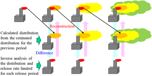
Figure 6. Inverse analysis domain setting. Green marks and arrows at the four corners of the domain indicated the locations and horizontal view angles of ETCCs. Examples of gamma-ray images at ETCC locations are also shown.

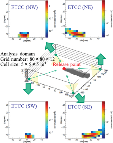
Figure 7. Hypothetical gamma-ray images by ETCCs located at (a) NW, (b) NE, (c) SW, and (d) SE corners of the analysis domain for the 622-keV gamma-ray of ¹³⁷Cs for the first 1-min period of the test case.

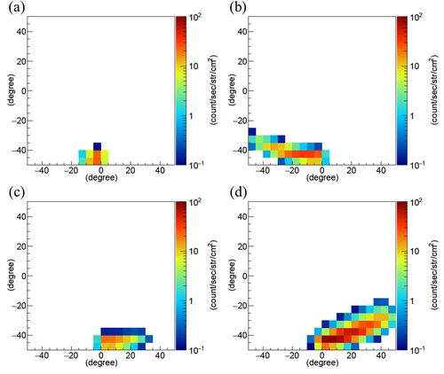
Figure 8. Scatterplots of air concentrations of ¹³⁷Cs comparing the ground truth with (a) the prior condition normalized by applying the release rate and (b) inverse analysis result of the optimum case for the first 1-min period of the test case. The solid and broken lines indicate the perfect and FAC2 lines, respectively.

Figure 9. Horizontal distributions of air concentrations of ¹³⁷Cs at the level of the release height for (a) the ground truth, (b) inverse analysis result of the optimum case, and (c) the prior condition normalized by applying the release rate for the first 1-min period of the test case.

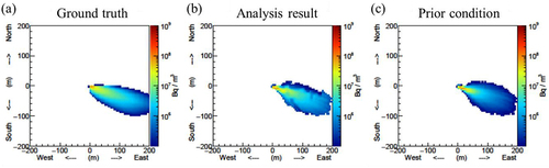
Table 1. Release rate and the maximum air concentration for the ground truth, the prior condition, and the inverse analysis results for 40 cases for the first 1-min period and FAC2 comparing air concentrations between the ground truth and analysis results.

Analysis case	Release rate (10^10 Bq s^−1)	Maximum concentration (10^7 Bq m^−3)	FAC2 (%)
The ground truth	1.000	7.290	-
The prior condition (normalized by applying the release rate)	1.000	8.246	27.74
I = 80, A = 0.1	1.113	9.729	39.93
I = 80, A = 0.2	1.087	9.603	43.37
I = 80, A = 0.5	1.060	9.165	48.66
I = 80, A = 1	1.043	8.535	51.68
I = 80, A = 2	1.031	7.714	53.49
I = 80, A = 5	1.028	7.237	54.16
I = 80, A = 10	1.029	7.225	54.13
I = 80, A = 20	1.033	7.661	53.95
I = 80, A = 50	1.039	7.645	51.27
I = 80, A = 100	1.045	7.957	47.92
I = 100, A = 0.1	1.104	9.717	42.33
I = 100, A = 0.2	1.075	9.575	46.54
I = 100, A = 0.5	1.048	9.090	52.60
I = 100, A = 1	1.039	8.422	55.17
I = 100, A = 2	1.033	7.539	55.28
I = 100, A = 5	1.033	7.199	55.05
I = 100, A = 10	1.033	7.329	55.43
I = 100, A = 20	1.032	7.524	54.10
I = 100, A = 50	1.039	7.566	52.15
I = 100, A = 100	1.049	8.026	48.94
I = 120, A = 0.1 I = 120, A = 0.2	1.096 1.064	9.706 9.547	43.84 49.58
I = 120, A = 0.5	1.039	9.022	54.50
I = 120, A = 1	1.032	8.315	55.79
I = 120, A = 2	1.030	7.384	54.66
I = 120, A = 5	1.032	7.146	54.06
I = 120, A = 10	1.030	7.247	54.35
I = 120, A = 20	1.029	7.328	52.46
I = 120, A = 50	1.038	7.411	50.58
I = 120, A = 100	1.051	7.926	47.38
I = 140, A = 0.1	1.089	9.696	45.22
I = 140, A = 0.2	1.057	9.520	51.72
I = 140, A = 0.5	1.034	8.960	54.91
I = 140, A = 1	1.030	8.221	55.24
I = 140, A = 2	1.030	7.260	52.79
I = 140, A = 5	1.032	7.110	52.38
I = 140, A = 10	1.030	7.125	51.80
I = 140, A = 20	1.031	7.183	49.95
I = 140, A = 50	1.042	7.345	46.92
I = 140, A = 100	1.057	7.876	44.51

Table 2. Release rate and the maximum air concentration for the second 1-min period by the ground truth and the inverse analysis results for the five cases, in which the release rates for the second 1-min period were 0.1, 0.5, 1.0, 2.0, and 10.0 times the release rate of the first 1-min period, together with FAC2 comparing air concentrations between the ground truth and analysis results.

Release rate change (times)	Release rate (10^10 Bq s^−1)		Maximum concentration (10^7 Bq m^−3)		FAC2 (%)
	The ground truth	Inverse analysis	The ground truth	Inverse analysis
0.1	0.100	0.539	0.862	1.872	2.83
0.5	0.500	0.945	4.353	4.662	23.99
1.0	1.000	1.469	8.459	9.678	28.88
2.0	2.000	2.499	17.980	21.124	30.25
10.0	10.000	10.606	85.216	103.713	28.04

Figure 10. Scatterplots of air concentrations of ¹³⁷Cs comparing the ground truth with the inverse analysis results for the cases with (a) 0.1, (b) 0.5, (c) 1.0, (d) 2.0, and (e) 10.0 times the release rate. The solid and broken lines indicate the perfect and FAC2 lines, respectively.

Table 3. Release rate and the maximum air concentration for the second 1-min period by the original and modified inverse analysis results for the five cases, in which the release rates for the second 1-min period were 0.1, 0.5, 1.0, 2.0, and 10.0 times the release rate of the first 1-min period, together with FAC2 comparing air concentrations between the original and modified analysis results.

Release rate change (times)	Release rate (10^10 Bq s^−1)		Maximum concentration (10^7 Bq m^−3)		FAC2 (%)
	Original analysis	Modified analysis	Original analysis	Modified analysis
0.1	0.539	0.620	1.872	2.427	88.18
0.5	0.945	0.984	4.662	4.762	91.34
1.0	1.469	1.505	9.678	8.966	94.38
2.0	2.499	2.536	21.124	21.047	96.29
10.0	10.606	10.636	103.713	103.834	99.63

Table 4. Characteristics of radionuclides, gamma-ray energies, emission rates, and attenuation coefficients in air for ¹³⁷Cs, ¹³⁴Cs, ¹³¹I, ¹³²I, ¹³³I, ¹³²Te, ¹³³Xe, and ⁸⁵Kr, and the maximum values of the hypothetical gamma-ray intensities by ETCC for these radionuclides generated using the same air concentration distribution for the first 1-min period.

Radionuclide	Gamma-ray energy (keV)	Emission rate (%)	Attenuation coefficient (cm^2 g^−1)	Maximum gamma-ray (count str^−1 sec^−1 cm^−2)
^137Cs	662	85.1	7.701 × 10^−2	98.8
^134Cs	605	97.6	8.025 × 10^−2	104.1
^131I	364	81.7	9.906 × 10^−2	53.2
^132I	955	17.6	6.500 × 10^−2	28.1
^133I	530	87.0	8.496 × 10^−2	82.0
^132Te	228	88.0	11.777 × 10^−2	35.2
^133Xe	81	38.0	16.550 × 10^−2	4.4
^85Kr	514	0.43	8.590 × 10^−2	0.4