Publication Cover
Molecular Physics
An International Journal at the Interface Between Chemistry and Physics
Volume 106, 2008 - Issue 8
279
Views
0
CrossRef citations to date
0
Altmetric
Errata

Erratum

Pages 1069-1091 | Received 21 Nov 2007, Accepted 27 Jan 2008, Published online: 24 Jul 2008

Figures & data

Figure 1. Diagram showing all of the relevant sites used in the calculation of , the intermolecular site–site distribution for a chosen pair of sites, ‘ia ' and ‘ja ' on two different molecules, each of species a. The sites ‘ia ' and ‘ja ' belong to ‘molecule 1' and ‘molecule 2' respectively, where, in the figure a dashed line is drawn between these two sites thus emphasizing the chosen site–site distribution, and, the distance, r i a j a , upon which it depends. (Note also that the choice of ia and ja leads to a specific for the case where the sites are ‘interior–end'.) At any fixed separation, r i a j a , the value of is influenced by the average positions of the other sites, ‘la ', on ‘molecule 1’, and, the other sites, ‘ma ', on ‘molecule 2’. also depends on the average behaviour of all of the other molecules in the fluid. This influence is incorporated by using a (freely ranging) representative third molecule, ‘molecule 3', containing the sites, ka . Further, for a mixed fluid, another representative third molecule must also be used to incorporate the influence of the other species, b. This molecule, also denoted as ‘molecule 3’, contains the sites, kb . In this diagram, the two species differ by the number of sites per chain, 3 for species a, and 4 for species b. (It is also noted that while the chains modelled in this work are tangent hard-spheres, the diagram above uses a common ball and stick representation.).
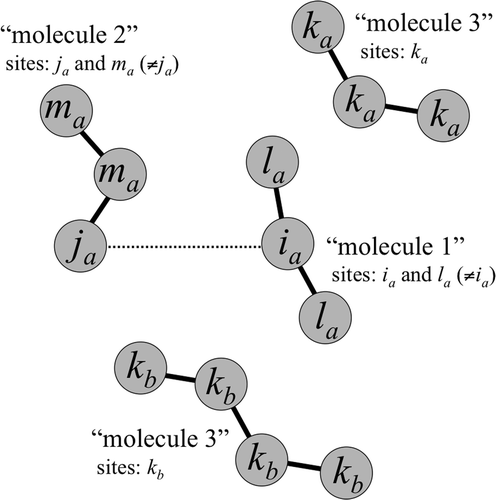
Figure 1. Diagram showing all of the relevant sites used in the calculation of , the intermolecular site–site distribution for a chosen pair of sites, ‘ia ' and ‘ja ' on two different molecules, each of species a. The sites ‘ia ' and ‘ja ' belong to ‘molecule 1' and ‘molecule 2' respectively, where, in the figure a dashed line is drawn between these two sites thus emphasizing the chosen site–site distribution, and, the distance, r i a j a , upon which it depends. (Note also that the choice of ia and ja leads to a specific for the case where the sites are ‘interior–end'.) At any fixed separation, r i a j a , the value of is influenced by the average positions of the other sites, ‘la ', on ‘molecule 1’, and, the other sites, ‘ma ', on ‘molecule 2’. also depends on the average behaviour of all of the other molecules in the fluid. This influence is incorporated by using a (freely ranging) representative third molecule, ‘molecule 3', containing the sites, ka . Further, for a mixed fluid, another representative third molecule must also be used to incorporate the influence of the other species, b. This molecule, also denoted as ‘molecule 3’, contains the sites, kb . In this diagram, the two species differ by the number of sites per chain, 3 for species a, and 4 for species b. (It is also noted that while the chains modelled in this work are tangent hard-spheres, the diagram above uses a common ball and stick representation.).

Figure 2. Diagram showing all of the relevant sites used in the calculation of , the intermolecular site–site distribution for a chosen pair of sites, ‘ia ' and ‘jb ' on two different molecules, one of species a, the other of species b. The diagram is similar to that in , except that now ‘molecule 2' is of species b, which contains the site jb , and the other sites mb . Again, in the mixed fluid, we must account for the case where ‘molecule 3' is of species a, and when it is of species b. See the caption of for other details.
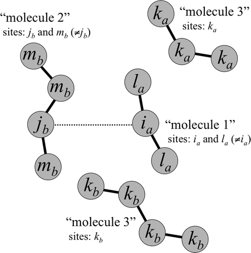
Figure 2. Diagram showing all of the relevant sites used in the calculation of , the intermolecular site–site distribution for a chosen pair of sites, ‘ia ' and ‘jb ' on two different molecules, one of species a, the other of species b. The diagram is similar to that in Figure 1, except that now ‘molecule 2' is of species b, which contains the site jb , and the other sites mb . Again, in the mixed fluid, we must account for the case where ‘molecule 3' is of species a, and when it is of species b. See the caption of Figure 1 for other details.

Figure 3. Average intermolecular site–site distribution functions () for tangent hard-sphere chain mixtures as calculated from CIE theory (lines) and MC simulation (symbols). Results in the upper panel are for a mixture of 3mers and 2mers at a density of η  = 0.2 and a composition of x 2mer  = x 3mer  = 0.5. Shown, respectively from top to bottom, are the distributions, , , and . In the lower panel, results are given for a mixture of 3mers and 1mers at a density of  η = 0.2 and a composition of x 1mer  = x 3mer  = 0.5. Shown are the distributions, , , and . (See the first paragraph of Section 3 for additional model details.)
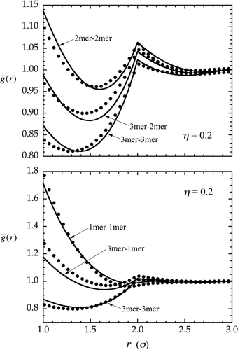
Figure 3. Average intermolecular site–site distribution functions () for tangent hard-sphere chain mixtures as calculated from CIE theory (lines) and MC simulation (symbols). Results in the upper panel are for a mixture of 3mers and 2mers at a density of η  = 0.2 and a composition of x 2mer  = x 3mer  = 0.5. Shown, respectively from top to bottom, are the distributions, , , and . In the lower panel, results are given for a mixture of 3mers and 1mers at a density of  η = 0.2 and a composition of x 1mer  = x 3mer  = 0.5. Shown are the distributions, , , and . (See the first paragraph of Section 3 for additional model details.)
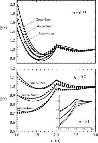
Figure 4. Average intermolecular site–site distribution functions () for a 4mer–2mer tangent hard-sphere chain mixture as calculated from CIE theory (lines) and MC simulation (symbols). Results are given at moderate density (η  = 0.2) in the lower panel, low density (η  = 0.1) in the inset, and at high density (η  = 0.35) in the upper panel, all cases corresponding to a composition of x 2mer  = x 4mer  = 0.5. Shown, respectively from top to bottom (at each density), are the distributions, , , and . (See the first paragraph of Section 3 for additional model details.)
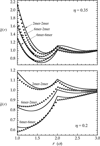
Figure 4. Average intermolecular site–site distribution functions () for a 4mer–2mer tangent hard-sphere chain mixture as calculated from CIE theory (lines) and MC simulation (symbols). Results are given at moderate density (η  = 0.2) in the lower panel, low density (η  = 0.1) in the inset, and at high density (η  = 0.35) in the upper panel, all cases corresponding to a composition of x 2mer  = x 4mer  = 0.5. Shown, respectively from top to bottom (at each density), are the distributions, , , and . (See the first paragraph of Section 3 for additional model details.)
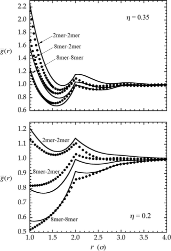
Figure 5. Average intermolecular site–site distribution functions () for a 6mer–2mer tangent hard-sphere chain mixture as calculated from CIE theory (lines) and MC simulation (symbols). Results are given at moderate density (η  = 0.2) in the lower panel, and at high density (η  = 0.35) in the upper panel, both cases corresponding to a composition of x 2mer  = x 6mer  = 0.5. Shown, respectively from top to bottom (at each density), are the distributions, , , and . (See the first paragraph of Section 3 for additional model details.)

Figure 5. Average intermolecular site–site distribution functions () for a 6mer–2mer tangent hard-sphere chain mixture as calculated from CIE theory (lines) and MC simulation (symbols). Results are given at moderate density (η  = 0.2) in the lower panel, and at high density (η  = 0.35) in the upper panel, both cases corresponding to a composition of x 2mer  = x 6mer  = 0.5. Shown, respectively from top to bottom (at each density), are the distributions, , , and . (See the first paragraph of Section 3 for additional model details.)

Figure 6. Average intermolecular site–site distribution functions () for an 8mer–2mer tangent hard-sphere chain mixture as calculated from CIE theory (lines) and MC simulation (symbols). Results are given at moderate density (η  = 0.2) in the lower panel, and at high density (η  = 0.35) in the upper panel, both cases corresponding to a composition of x 2mer  = x 8mer  = 0.5. Shown, respectively from top to bottom (at each density), are the distributions, , , and . (See the first paragraph of Section 3 for additional model details.)

Figure 6. Average intermolecular site–site distribution functions () for an 8mer–2mer tangent hard-sphere chain mixture as calculated from CIE theory (lines) and MC simulation (symbols). Results are given at moderate density (η  = 0.2) in the lower panel, and at high density (η  = 0.35) in the upper panel, both cases corresponding to a composition of x 2mer  = x 8mer  = 0.5. Shown, respectively from top to bottom (at each density), are the distributions, , , and . (See the first paragraph of Section 3 for additional model details.)

Figure 7. Specific intermolecular site–site distribution functions for a 4mer–2mer tangent hard-sphere chain mixture at moderate density (η  = 0.2) and a composition of x 2mer  = x 4mer  = 0.5. Results in the upper panel are given for the specific distributions, , involving the 4mer–4mer molecular pair (where ‘a'  = 4mer). In this case there are three distinct distributions: the ‘end–end' distribution (e.g. ia  = 1 or 4, and ja  = 1 or 4) given as long-dashed lines (CIE) and triangles (MC), the ‘middle–middle' distribution (e.g. ia  = 2 or 3, and ja  = 2 or 3) given as short-dashed lines (CIE) and diamonds (MC), and the ‘end–middle' distribution (e.g. ia  = 1 or 4, and ja  = 2 or 3) given as solid lines (CIE) and circles (MC). Results in the lower panel are for the two distinct distributions, , involving the 4mer–2mer pair (where ‘b'  = 2mer). These are: the ‘end' distribution involving the end of the 4mer (ia  = 1 or 4; the sites jb are equivalent) given as long-dashed lines (CIE) and triangles (MC), and the ‘middle' distribution (ia  = 2 or 3) given as short-dashed lines (CIE) and diamonds (MC), and the end–middle distribution. (See the first paragraph of Section 3 for additional model details.)
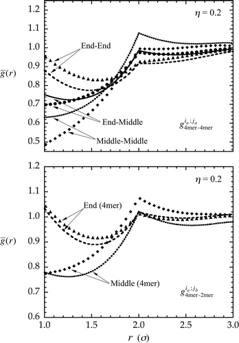
Figure 7. Specific intermolecular site–site distribution functions for a 4mer–2mer tangent hard-sphere chain mixture at moderate density (η  = 0.2) and a composition of x 2mer  = x 4mer  = 0.5. Results in the upper panel are given for the specific distributions, , involving the 4mer–4mer molecular pair (where ‘a'  = 4mer). In this case there are three distinct distributions: the ‘end–end' distribution (e.g. ia  = 1 or 4, and ja  = 1 or 4) given as long-dashed lines (CIE) and triangles (MC), the ‘middle–middle' distribution (e.g. ia  = 2 or 3, and ja  = 2 or 3) given as short-dashed lines (CIE) and diamonds (MC), and the ‘end–middle' distribution (e.g. ia  = 1 or 4, and ja  = 2 or 3) given as solid lines (CIE) and circles (MC). Results in the lower panel are for the two distinct distributions, , involving the 4mer–2mer pair (where ‘b'  = 2mer). These are: the ‘end' distribution involving the end of the 4mer (ia  = 1 or 4; the sites jb are equivalent) given as long-dashed lines (CIE) and triangles (MC), and the ‘middle' distribution (ia  = 2 or 3) given as short-dashed lines (CIE) and diamonds (MC), and the end–middle distribution. (See the first paragraph of Section 3 for additional model details.)

Figure 8. Average intermolecular site–site distribution functions () for a 4mer–2mer tangent hard-sphere chain mixture at varied compositions (x 2mer  = 0.1 and x 2mer  = 0.9). Results are given for CIE theory (lines) and MC simulation (symbols) at a density of η  = 0.2, and, in the inset, at η  = 0.35. Shown for η  = 0.2, are the distributions, , , and , where, in all cases, the upper (higher valued) curve is for the mixture at x 2mer  = 0.1, and the lower curve is for x 2mer  = 0.9. At η  = 0.35, again, CIE and MC both predict all distributions to be higher valued for the case of x 2mer  = 0.1. Here, only the distribution, , is shown to avoid clutter in the figure. (See the first paragraph of Section 3 for additional model details.)
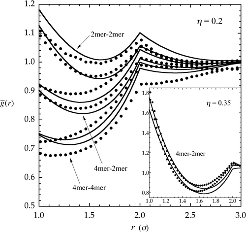
Figure 8. Average intermolecular site–site distribution functions () for a 4mer–2mer tangent hard-sphere chain mixture at varied compositions (x 2mer  = 0.1 and x 2mer  = 0.9). Results are given for CIE theory (lines) and MC simulation (symbols) at a density of η  = 0.2, and, in the inset, at η  = 0.35. Shown for η  = 0.2, are the distributions, , , and , where, in all cases, the upper (higher valued) curve is for the mixture at x 2mer  = 0.1, and the lower curve is for x 2mer  = 0.9. At η  = 0.35, again, CIE and MC both predict all distributions to be higher valued for the case of x 2mer  = 0.1. Here, only the distribution, , is shown to avoid clutter in the figure. (See the first paragraph of Section 3 for additional model details.)

Figure 9. Average intermolecular site–site distribution, , in a series of hard-sphere chain mixtures as calculated from CIE theory (lines) and MC simulation (symbols). All mixtures contain the 2mer species at a composition of x 2mer  = 0.5. Also included is the pure 2mer fluid. The density in all cases is η  = 0.2. The distributions, , for both CIE and MC, are ordered in the same way, where, from top to bottom, the curves correspond respectively to the mixtures, 8mer–2mer, 6mer–2mer, 4mer–2mer, 3mer–2mer, and pure 2mer. (See the first paragraph of Section 3 for additional model details.)
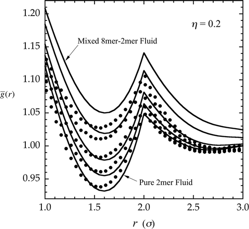
Figure 9. Average intermolecular site–site distribution, , in a series of hard-sphere chain mixtures as calculated from CIE theory (lines) and MC simulation (symbols). All mixtures contain the 2mer species at a composition of x 2mer  = 0.5. Also included is the pure 2mer fluid. The density in all cases is η  = 0.2. The distributions, , for both CIE and MC, are ordered in the same way, where, from top to bottom, the curves correspond respectively to the mixtures, 8mer–2mer, 6mer–2mer, 4mer–2mer, 3mer–2mer, and pure 2mer. (See the first paragraph of Section 3 for additional model details.)

Reprints and Corporate Permissions

Please note: Selecting permissions does not provide access to the full text of the article, please see our help page How do I view content?

To request a reprint or corporate permissions for this article, please click on the relevant link below:

Academic Permissions

Please note: Selecting permissions does not provide access to the full text of the article, please see our help page How do I view content?

Obtain permissions instantly via Rightslink by clicking on the button below:

If you are unable to obtain permissions via Rightslink, please complete and submit this Permissions form. For more information, please visit our Permissions help page.