Asymptotic behaviour of the electron density and the Kohn–Sham potential in case of a Kohn–Sham HOMO nodal plane

Figures & data

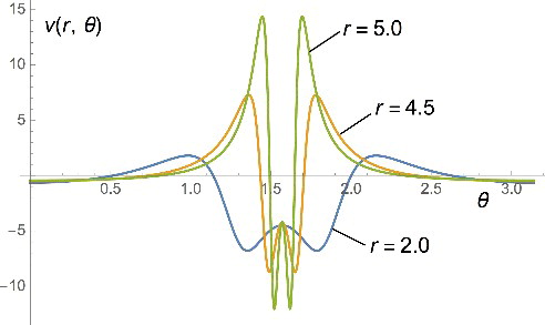
Figure 1. The large-r behaviour of the potential that generates the orbital with the asymptotic behaviour of Equation (5(5) $$\psi \left(\mathbf{r}\right)\sim e^{-r}\left(cos{\left(\theta \right)}^2+\frac{1}{r^2}\right),$$(5) ) as a function of r and the azimuthal angle θ = arccos(z/r). We clearly see that this potential has a ‘ridge’ on the xy plane (corresponding to θ = π/2), where it goes asymptotically to a constant. The ‘ridge’ shrinks as r gets larger and larger. Despite this constant, the orbital has the same exponential decay everywhere, it only decays 1/r² faster on the plane.

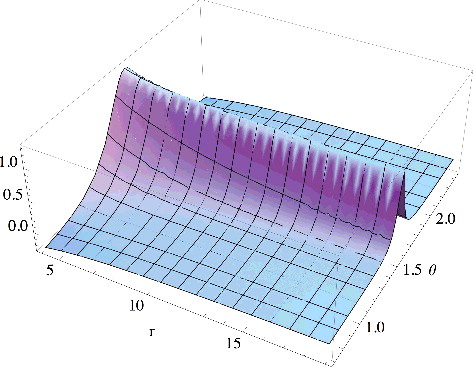
Figure 2. The large-r behaviour of the potential that generates the orbital with the asymptotic behaviour of Equation (6(6) $$\psi \left(\mathbf{r}\right)\sim e^{-r}cos{\left(\theta \right)}^2+e^{-2r}.$$(6) ) as a function of r and the azimuthal angle θ = arccos(z/r). We clearly see that this potential has a ‘ridge’ on the xy plane (corresponding to θ = π/2), where it diverges exponentially. The ‘ridge’ shrinks as r gets larger and larger.

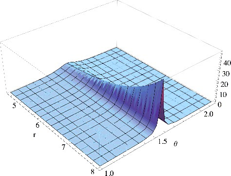
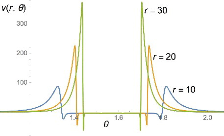
Figure 3. The potential v(r, θ) that generates the orbital with the asymptotic behaviour of Equation (34(34) $${\psi }_{s,H-1}(r,\theta )=\frac{e^{-3r}}{{cos}^4\theta +e^{-2r}}$$(34) ), shown as a function of the azimuthal angle $\theta =arccos(z/r)$, for different values of r. We see that although on the plane the potential goes to a negative constant, its most prominent features are actually very high positive peaks close to the plane. The region delimited by the peaks becomes very narrow (the peaks become true spikes) when r → ∞, while their height grows exponentially with r.

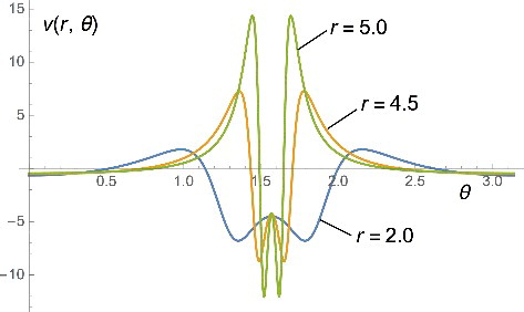
Figure 4. The potential v(r, θ) that generates the orbital with the asymptotic behaviour of Equation (30(30) $$\begin{array}{cc}& {\psi }_{s,H-1}(r\to \infty ,\theta )\to \frac{e^{-\sqrt{2I_1}r}}{f(cos\theta )+C{e}^{-(\sqrt{2I_1}-\sqrt{2I_0})r}}\hfill \\ & =\frac{1}{e^{\sqrt{2I_1}r}f(cos\theta )+C{e}^{-\sqrt{2I_0}r}}\hfill \end{array}$$(30) ) with f(cos θ) = cos²θ, shown as a function of r and of the azimuthal angle $\theta =arccos(z/r)$. We see that as r increases, the potential tends exponentially fast to −∞ on the nodal plane, corresponding to θ = π/2.

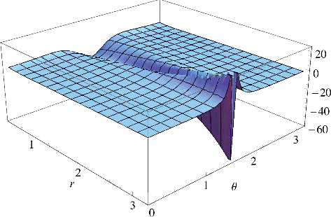
Figure 5. The potential v(r, θ) that generates the orbital with the asymptotic behaviour of Equation (30(30) $$\begin{array}{cc}& {\psi }_{s,H-1}(r\to \infty ,\theta )\to \frac{e^{-\sqrt{2I_1}r}}{f(cos\theta )+C{e}^{-(\sqrt{2I_1}-\sqrt{2I_0})r}}\hfill \\ & =\frac{1}{e^{\sqrt{2I_1}r}f(cos\theta )+C{e}^{-\sqrt{2I_0}r}}\hfill \end{array}$$(30) ) with f(cos θ) = exp(− 1/cos ²θ), shown as a function of the azimuthal angle $\theta =arccos(z/r)$, for different values of r. We see that now the region close to the plane where the potential goes to a negative constant is larger than the one of Figure 3. Yet, this region eventually shrinks as r → ∞, similarly to the case of Figure 3.