Structure and equation-of-state of a disordered system of shape anisotropic patchy particles

Figures & data

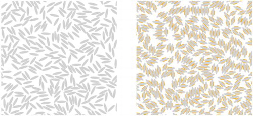
Figure 1. Schematic figure visualising the geometric definition of the patches in our model. For reasons of clarity only two of the up to four patches are shown; they can be positioned at the (co-)vertices of the elliptic body. The impenetrable, elliptic particle is defined via its semi-axes a and b; for this particular representation a value $\kappa =a/b=2$ was assumed. The osculating circles of the (co-)vertices with radii $r_a$ and $r_b$ are marked by the pink lines. The patches (highlighted in pink) are approximated by sectorial regions of two concentric circles: the inner one is the osculating circle of the respective (co-)vertex while the outer circle has a radius which is by ${\delta }_a$ or ${\delta }_b$ larger than $r_a$ or $r_b$, defining thus the interaction range of the patch. Inside the patch region the interaction is assumed to be constant. The widths of the patches are measured by the opening angles ${\theta }_a$ and ${\theta }_b$ (as seen from the centres of the osculating circles) or ${\phi }_a$ and ${\phi }_b$ (as seen from the centre of the ellipse).

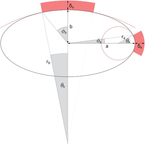
Table 1. Values that specify the maximum extent of patches in our model, as specified by a criterion put forward in the text: ${\theta }_{a,\max }$ and ${\theta }_{b,\max }$ – maximum opening angles of the patches as seen from the centres of the respective osculating circles, ${\phi }_{a,\max }$ and ${\phi }_{b,\max }$ – maximum opening angles of the patches as seen from the centre of the ellipse, and $p_a$ and $p_b$ – maximum patch extents as measured in units of the elliptic circumference.

		${\theta }_{a,\max }$	${\theta }_{b,\max }$	${\phi }_{a,\max }$	${\phi }_{b,\max }$	$p_a$	$p_b$
$\kappa =2$	ε = 0.1 %	${29.30}^{\circ }$	${11.77}^{\circ }$	${7.20}^{\circ }$	${41.69}^{\circ }$	0.11	0.36
	ε = 0.5 %	${45.29}^{\circ }$	${17.28}^{\circ }$	${10.86}^{\circ }$	${55.40}^{\circ }$	0.17	0.53
$\kappa =4$	ε = 0.1 %	${36.71}^{\circ }$	${6.03}^{\circ }$	${2.17}^{\circ }$	${61.51}^{\circ }$	0.04	0.40
	ε = 0.5 %	${57.60}^{\circ }$	${8.76}^{\circ }$	${3.11}^{\circ }$	${71.55}^{\circ }$	0.06	0.59
$\kappa =6$	ε = 0.1 %	${43.05}^{\circ }$	${4.17}^{\circ }$	${1.09}^{\circ }$	${70.96}^{\circ }$	0.02	0.43
	ε = 0.5 %	${67.97}^{\circ }$	${6.04}^{\circ }$	${1.50}^{\circ }$	${78.08}^{\circ }$	0.03	0.62

Note: Representative values for these quantities are given for the three aspect ratios κ (as they are considered in this study) and for two different values of ε, used as a tolerance in the aforementioned criterion.

Figure 2. Schematic representations of elliptic patchy particles as they have been used in this contribution; patches are highlighted in orange. Particles with aspect ratios $\kappa =2,4$ (panels a and b), and 6 (panel c) have been considered. In all cases the interaction range was chosen to be ${\delta }_b=0.1$ (in units of $2\sqrt{ab}$); the opening angles ${\theta }_b={11.77}^{\circ },{6.03}^{\circ }$ (panels a and b) and ${4.17}^{\circ }$ (panel c) are chosen such that the criterion for approximating the ellipse by its osculating circle within the patch region is fulfilled with an accuracy of $\epsilon =0.1\mathrm{\%}$ (see text and Table 1).

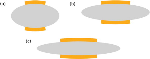
Figure 3. Representative snapshots taken from our NPT MC simulations, showing particles in a section of the simulation cell. Results have been obtained for patchy elliptic particles with aspect ratio $\kappa =2$ and reduced, dimensionless pressure $P^{\star }=2$. Selected temperatures are: $T^{\star }=\mathrm{\infty }$ – top left, $T^{\star }=2.0$ – top right, $T^{\star }=1.0$ – bottom left, and $T^{\star }=0.6$ – bottom right.

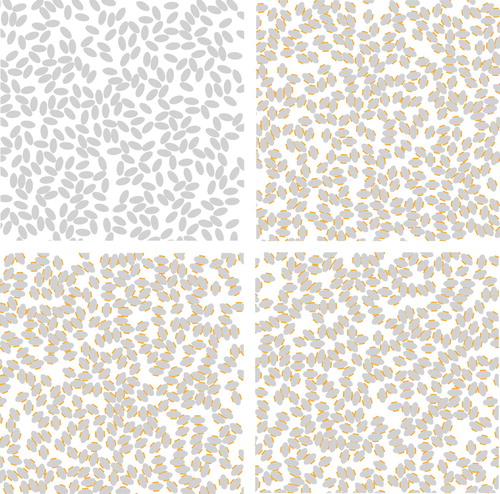
Figure 4. Representative snapshots taken from our NPT MC simulations, showing particles in a section of the simulation cell. Results have been obtained for patchy elliptic particles with aspect ratio $\kappa =4$ and reduced, dimensionless pressure $P^{\star }=2$. Selected temperatures are: $T^{\star }=\mathrm{\infty }$ – top left, $T^{\star }=2.0$ – top right, $T^{\star }=1.0$ – bottom left, and $T^{\star }=0.6$ – bottom right.

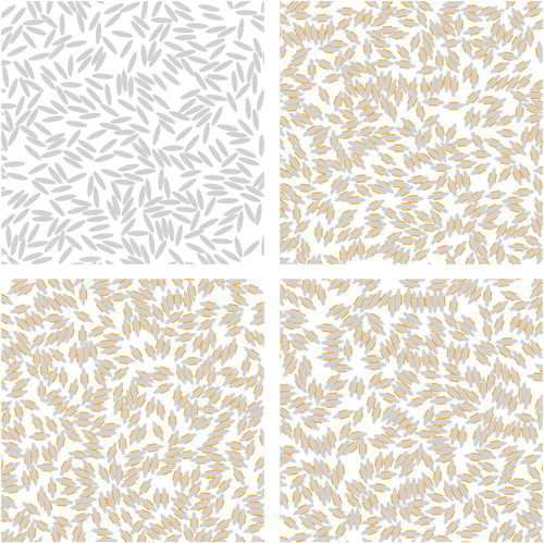
Figure 5. Representative snapshots taken from our NPT MC simulations, showing particles in a section of the simulation cell. Results have been obtained for patchy elliptic particles with aspect ratio $\kappa =6$ and reduced, dimensionless pressure $P^{\star }=2$. Selected temperatures are: $T^{\star }=\mathrm{\infty }$ – top left, $T^{\star }=2.0$ – top right, $T^{\star }=1.0$ – bottom left, and $T^{\star }=0.6$ – bottom right.

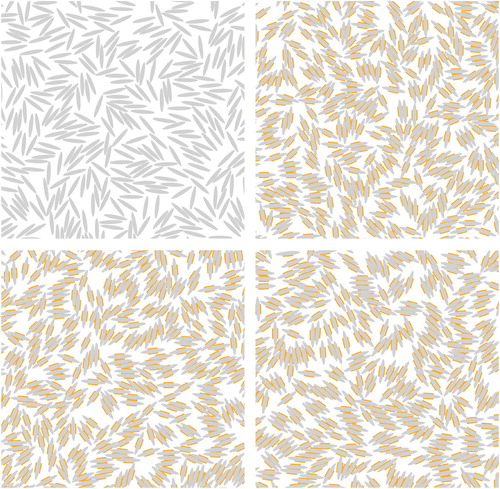
Figure 6. Radial distribution functions $g\left(r\right)$ as functions of r (in reduced units of $2\sqrt{ab}$) for κ- and $P^{\star }$-values as specified on top of each panel and for different temperatures (as labelled in the panels). The vertical arrows in each of the panels indicate for the respective κ-values the distances r = 2a and r = 2b (again in reduced units $2\sqrt{ab}$).

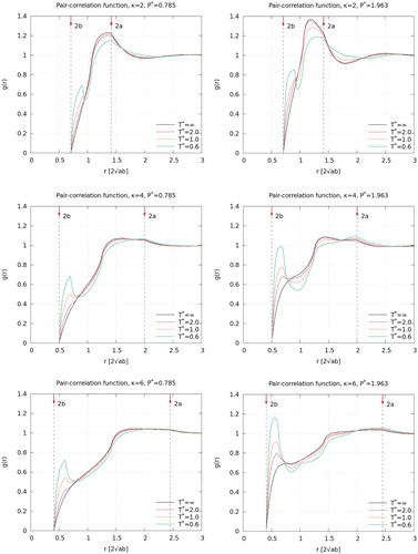
Figure 7. Equation-of-state, i.e. $P^{\star }$ as a function of the packing fraction η for four different temperatures (as labelled), including the case of undecorated, hard ellipses (i.e. for $T^{\star }=\mathrm{\infty }$; in the latter case our results are consistent with the data presented in [9]. Results are shown for three different κ-values: top panel – $\kappa =2$, central panel – $\kappa =4$, and bottom panel – $\kappa =6$. The insets show the trivial low-density equation-of-state of the system.

J. Cuesta and D. Frenkel, Phys. Rev. A 42, 2126 (1990). doi: 10.1103/PhysRevA.42.2126

 PubMed Web of Science ®Google Scholar