Excitation of H₂ at large internuclear separation: outer well states and continuum resonances

Figures & data

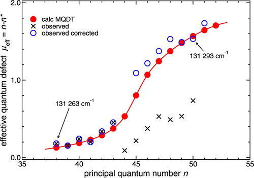
Figure 1. Level scheme with potential energy curves for H${}_2$ and the three-laser excitation pathway. The first laser, photolysing H${}_2$S, produces high-v levels in the electronic ground state; the second laser induces the F−X transitions; the third laser ionises the molecule at energies above 131,000 cm⁻¹. All excitations occur at the large internuclear separation $R=$4–5 a.u, indicated by the grey (yellow) shaded bar. See text for further details.

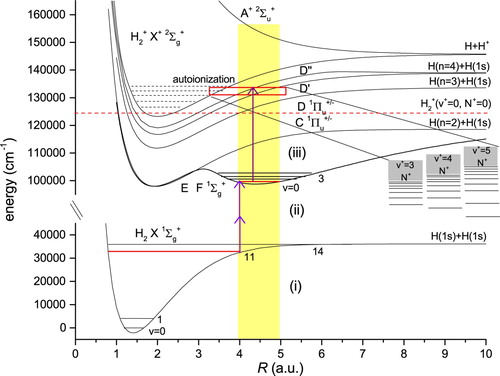
Figure 2. Experimental configuration. Pulsed dye laser (PDL I) provides UV pulses for photolysis of H${}_2$S molecules. The nascent H${}_2^{\ast }\left(v\right)$ photoproducts are subjected to two-photon Doppler-free spectroscopy, using 305 nm pulses generated by an injection-seeded narrowband PDA laser. A third laser (PDL II) is employed for recording autoionisation resonances excited from the F outer well levels. Ions are extracted by the electrostatic lens and detected at the end of the time-of-flight (TOF) tube after mass-selection.

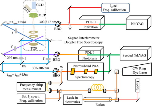
Figure 3. Doppler-free two-photon recording of the $Q\left(7\right)$ line calibrated using etalon markers with an FSR of 300.01 MHz and with respect to a reference $(B-X)P\left(94\right)(12,3)a15$ hyperfine line of ¹²⁷I${}_2$ at 16,377.60438 cm⁻¹ [42].

Figure 4. (a) Recorded spectra of the $F-X(0,11)$ $Q\left(7\right)$ line under various power densities; (b) ac-Stark extrapolation plot of the $Q\left(7\right)$ transition for determining the field-free value of the transition frequency.

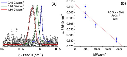
Table 1. Results of high precision measurements on two transitions in the $F-X(0,11)$ band. The experimentally-derived level energies are compared with the results from MQDT calculations for the F state [9]. Values are given in cm⁻¹.

		$F(v=0)$ Level energy
$J^{″}$	Q($J^{″}$) Transition energy${}^{\mathrm{a}}$	Exp${}^{\mathrm{b}}$	Calc [9]	Difference Exp-Calc
6	65,731.2825 (20)	99,619.7840 (57)	99,621.16	$-1.38$
7	65,510.6124 (20)	99,704.6413 (56)	99,706.04	$-1.40$

${}^{\mathrm{a}}$Transition frequencies measured in this experiment.

${}^{\mathrm{b}}$Level energies are deduced using calculated energies of $X(v=11,J^{″})$ taken from Komasa et al. [31].

Figure 5. Autoionisation spectra recorded from $F^1{\mathrm{\Sigma }}_g^{+}(v=0)$, $J^{\prime }=4$ and $J^{\prime }=6$ states in para-H${}_2$. Common resonances with J=5 calculated from MQDT are indicated.

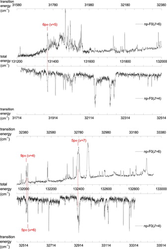
Figure 6. Autoionisation spectra recorded from $F^1{\mathrm{\Sigma }}_g^{+}(v=0)$, $J^{\prime }=5$ and $J^{\prime }=7$ states in ortho-H${}_2$. Common resonances with J=6 calculated from MQDT are indicated. The ($v^{+}=3,N^{+}=3$) limit of the complex resonance Rydberg series is also shown.

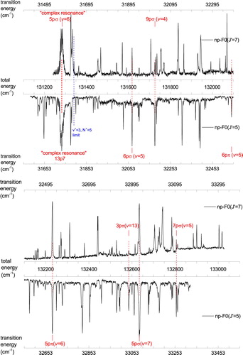
Figure 7. Complex resonance in ortho-H${}_2$ recorded from both $F^1{\mathrm{\Sigma }}_g^{+}(v=0)$, $J^{\prime }=5$ and $J^{\prime }=7$ intermediate states. The vertical lines indicate members of an np Rydberg series converging to a limit with $v^{+}=3$ and $N^{+}=5$ at 131,339.66 cm⁻¹. The red circles represent the calculated level energies, numbered consecutively from n=36, i.e. including interlopers. The approximate weight of the $5p\sigma ,v=6,J=6$ interloper in the wave function of each level is indicated on the ordinate and provides a rough measure of the intensity transferred from the interloper to the Rydberg series. Another interloper $13p,v^{+}=3,N^{+}=7$ is also identified in the MQDT analysis as explained in the main text.

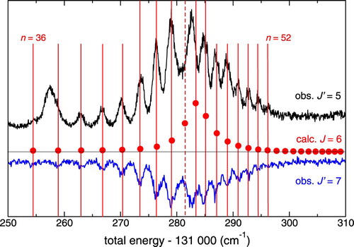
Table 2. Autoionisation resonances for J=5 and J=6 angular momenta observed in the spectra of Figures 5 and 6, here assigned and compared with calculations via MQDT theory. Values are given in cm⁻¹.

J	Resonance	Resonance energy Observed	Resonance energy Calculated	Resonance width Γ Calculated
5	$6p\sigma ,v=5$	131,370	131,375	0.3
5	$9p\pi ,v=4$	132,019	132,020	1.0
5	$5p\pi ,v=6$	132,030	132,030	0.8
5	$5p\sigma ,v=7$	132,394	132,393	6.6
6	$13p7,v=3^{\mathrm{a}}$	–	131,281	–
6	$5p\sigma ,v=6^{\mathrm{a}}$	131,281	131,283	0.3${}^{\mathrm{b}}$
6	$6p\sigma ,v=5$	131,617	131,619	0.4
6	$9p\sigma ,v=4$	131,726	131,726	1.2
6	$6p\pi ,v=5$	132,091	132,092	0.5
6	$5p\pi ,v=6$	132,231	132,233	0.2
6	$3p\pi ,v={13}^{\mathrm{c}}$	132,585	132,585	–
6	$5p\sigma ,v=7$	132,634	132,633	1.3
6	$7p\sigma ,v=5$	132,806	132,808	0.4

${}^{\mathrm{a}}$Interlopers in the complex resonance plotted in Figure 7.

${}^{\mathrm{b}}$Width of the components near the centre. The width of the whole group is calculated to be $\sim 8$ cm⁻¹.

${}^{\mathrm{c}}$Tentative assignment.

Figure 8. Effective quantum defects derived from the observed peaks in Figure 7. The MQDT analysis reveals the presence of two interlopers in this complex resonance, see text for details.

S. Xu, R. van Dierendonck, W. Hogervorst and W. Ubachs, J. Mol. Spectr. 201, 256 (2000). doi: 10.1006/jmsp.2000.8085

 PubMed Web of Science ®Google Scholar

G.D. Dickenson, E.J. Salumbides, M. Niu, Ch. Jungen, S.C. Ross and W. Ubachs, Phys. Rev. A 86, 032502 (2012). doi: 10.1103/PhysRevA.86.032502

 Web of Science ®Google Scholar

J. Komasa, K. Piszczatowski, G. Łach, M. Przybytek, B. Jeziorski and K. Pachucki, J. Chem. Theory Comput. 7, 3105–3115 (2011). doi: 10.1021/ct200438t

 PubMed Web of Science ®Google Scholar