Machine learning for collective variable discovery and enhanced sampling in biomolecular simulation

Figures & data

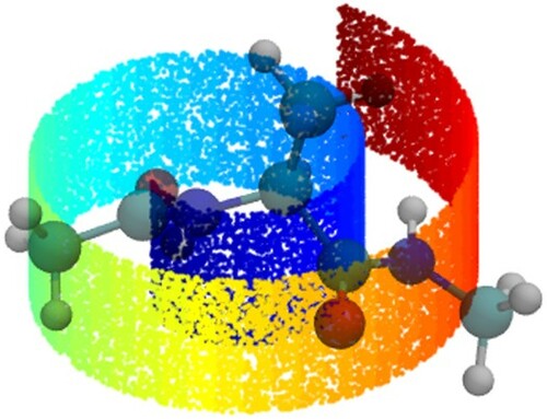
Figure 1. Schematic diagram of a three-layer fully-connected feed-forward neural network. The output of neuron i from layer k is denoted $y_i^k$ and the bias node for layer k denoted $b^k$. The arrows connecting pairs of neurons are the trainable weights $w_{ji}$. The output of each layer is computed from a weighted sum of outputs of the previous layer passed through a nonlinear activation function (Equation (1(1) $y_i^k=f(\sum _{j=1}^N{w}_{ji}^k{y}_j^{k-1}+b_i^k),$(1) )). (Image constructed using code downloaded from http://www.texample.net/tikz/examples/neural-network with the permission of the author Kjell Magne Fauske.)

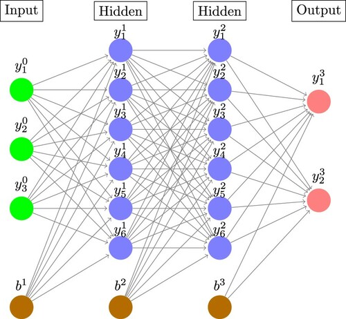
Figure 2. Schematic diagram of the Markov state model (MSM) construction and analysis pipeline. (a) Many short molecular dynamics trajectories are collected. (b) The snapshots constituting each trajectory are featurized, projected into a low-dimensional space, and clustered into microstates. Each frame in each trajectory is assigned to a microstate. For illustrative purposes, four microstates are considered and coloured green, blue, purple, and pink. (c) Counting the number of transitions between microstates furnishes the transition counts matrix. (d) Assuming the system is at equilibrium and therefore follows detailed balance, the count matrix is symmetrised and normalised to generate the reversible transition matrix defining the conditional transition probabilities between microstates. (e) The equilibrium distribution over microstates is furnished by the leading eigenvector of the transition probability matrix, here illustrated in a pie chart. States with greater populations are more thermodynamically stable. (f) The higher eigenvectors correspond to a hierarchy of increasingly fast dynamical relaxations over the microstates. The first of these possess a negative entry corresponding to the green state and positive entries for the other states, therefore characterising the net transport of probability distribution out of the green microstate and into the blue, purple, and pink. If desired, the microstates can be further coarse grained into macrostates, typically by clustering of the microstate transition matrix. Image reprinted with permission from Ref. [20]. Copyright (2018) American Chemical Society.

Figure 3. Schematic illustration of iMapD. The curved teal sheet is a cartoon representation of a low-dimensional manifold residing within the high-dimensional coordinate space of the molecular system (black background) and to which the system dynamics are effectively restrained. This manifold supports the low-dimensional molecular free energy surface of system (red contours denote potential wells). The dimensionality of the manifold, good collective variables with which to parameterise it, and topography of the free energy surface are a priori unknown. iMapD commences by running short unbiased simulations to perform local exploration of the underlying manifold and which define an initial cloud of points $C^{(1)}$. Boundary points are identified, here $B{P}_1^{(1)}$ and $B{P}_2^{(1)}$, and local PCA applied to define a locally-linear approximation to the manifold geometry that is locally valid in the vicinity of each point. An outward step is then taken within these linear subspaces, here from $B{P}_1^{(1)}$ to expand the exploration frontier. The projected point may lie off the manifold due to the linear approximation inherent in the outward projection and so a short ‘lifting’ operation is employed to relax it back to the manifold. This point then seeds a new unbiased simulation that generates a new cloud of points $C^{(2)}$ and the process is repeated until the manifold is fully explored. In this manner iMapD explores the manifold by ‘walking on clouds’. Image adapted with permission from Ref. [63].

Figure 4. Schematic illustration of SandCV. Molecular configurations $\mathbf{r}$ are aligned to a reference configuration $\mathcal{A}(\mathbf{r})$ then projected onto the Isomap manifold using a nearest neighbour projection and a basis function expansion in a number of landmark points ${\mathcal{M}}^{-1}\circ \mathcal{P}(\mathbf{x})$. Enhanced sampling using adaptive biasing force (ABF) is effected by propagating biasing forces over the manifold $\mathbf{F}(\mathit{\xi })$ into forces on atoms $\mathbf{F}(\mathbf{r})$ through the Jacobian of the explicit and differentiable composite mapping function $\mathcal{C}(\mathbf{r})={\mathcal{M}}^{-1}\circ \mathcal{P}\circ \mathcal{A}(\mathbf{r})$. Image reprinted from Ref. [39], with the permission of AIP Publishing.

Figure 5. Molecular enhanced sampling with autoencoders (MESA). An autoencoding neural network (autoencoder) is trained to reconstruct molecular configurations via a low-dimensional latent space where the CVs are defined by neuron activations within the bottleneck layer. The encoder ${\mathrm{\Theta }}_{\mathrm{proj}}$ performs the low-dimensional projection from molecular coordinates $\mathbf{z}$ in the high dimensional atomic coordinate space $\mathcal{H}$ into the low-dimensional latent space $\mathcal{L}$ and the decoder ${\mathrm{\Theta }}_{\mathrm{rec}}$ performs the approximate reconstruction back to $\hat{\mathbf{z}}$. The encoder furnishes, by construction, an exact, explicit, and differentiable mapping from the atomic coordinates to CVs that can be modularly incorporated into any off-the-shelf CV biasing enhanced sampling technique.

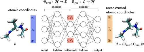
Figure 6. Block diagram of a time-lagged autoencoder (TAE). The encoder projects a molecular configuration ${\mathbf{z}}_t$ at time t into a low-dimensional latent embedding ${\mathbf{e}}_t$ from which a time-lagged molecular configuration ${\mathbf{z}}_{t+\tau }$ at time $(t+\tau )$ is subsequently reconstructed. For τ = 0 the TAE reduces to a standard AE and the CV discovery process is equivalent to MESA (Section 3.3). Image reprinted from Ref. [108], with the permission of AIP Publishing.

Figure 7. State-free reversible VAMPnets. Pairs of time-lagged molecular configurations $\{\mathbf{x}(t),\mathbf{x}(t+\tau )\}$ are featurized and transformed by a twin-lobe ANN into a space of nonlinear basis functions $\{\mathit{\zeta }(\mathbf{x}(t)),\mathit{\zeta }(\mathbf{x}(t+\tau ))\}$. These basis functions are employed within a linear VAC to furnish approximations $\tilde{\mathit{\psi }}$ to the leading eigenfunctions of the transfer operator. The twin-lobed ANN is trained to maximise a VAMP-r score measuring the cumulative kinetic variance explained and which reaches a maximum when the eigenfunction approximations are coincident with the true eigenfunctions of the transfer operator.

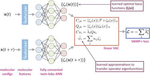
Figure 8. Deep Generative MSM (DeepGenMSM) and the ‘rewiring trick’. (left) The encoder $\mathit{\chi }(\mathbf{x})$ within the twin-lobe ANN is trained to learn mappings of molecular configurations $\mathbf{x}$ to probabilistic memberships $\mathbf{y}$ of one of m macrostates. The generator is trained against the learned ‘landing probabilities’ $q_i(\mathbf{z};\tau )$ that a system prepared in macrostate i will transition to molecular configuration $\mathbf{z}$ after a time τ. (right) The rewiring trick reconnects the generator and encoder to furnish a valid estimate $\tilde{\mathbf{K}}$ for the MSM transition matrix between the embedding into the m discrete states learned by the encoder. Image adapted from Ref. [135], with permission from the author Prof. Frank Noé (Freie Universität Berlin).

Table 1. Software packages and libraries available for some of the collective variable discovery and enhanced sampling techniques discussed in this review.

Method	Software Packages
ANNs	Keras (keras.io)
	TensorFlow (www.tensorflow.org)
	PyTorch (pytorch.org)
DMAPS	github.com/hsidky/dmaps
	github.com/DiffusionMapsAcademics/ pyDiffMap
MSM, TICA	PyEmma (www.emma-project.org/latest/)
	MSMBuilder (msmbuilder.org/)
MESA	github.com/weiHelloWorld/accelerated_ sampling_with_autoencoder
TAE, VAMPnets	github.com/markovmodel/deeptime
VDE	github.com/msmbuilder/vde
SRV	github.com/hsidky/srv
DeepGenMSM	github.com/markovmodel/deep_gen_msm
Enhanced Sampling Suites	SSAGES (github.com/MICCoM/SSAGES-public)
	PLUMED (www.plumed.org)
	Colvars (colvars.github.io)

B.E. Husic and V.S. Pande, J. Am. Chem. Soc. 140 (7), 2386–2396 (2018).

 PubMed Web of Science ®Google Scholar

E. Chiavazzo, R. Covino, R.R. Coifman, C.W. Gear, A.S. Georgiou, G. Hummer and I.G. Kevrekidis, Proc. Natl. Acad. Sci. 114 (28), E5494–E5503 (2017).

 PubMed Web of Science ®Google Scholar

B. Hashemian, D. Millán and M. Arroyo, J. Chem. Phys. 139 (21), 12B601_1 (2013).

 Web of Science ®Google Scholar

C. Wehmeyer and F. Noé, J. Chem. Phys. 148 (24), 241703 (2018).

 PubMed Web of Science ®Google Scholar

H. Wu, A. Mardt, L. Pasquali, and F. Noé, 2018, in Advances in Neural Information Processing Systems, pp. 3975–3984.

 Google Scholar