Automated determination of hybrid particle-field parameters by machine learning

Figures & data

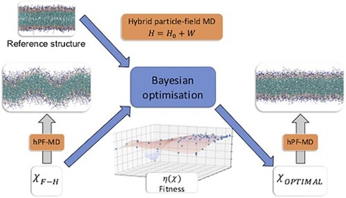
Figure 1. Protocol for optimising hPF force fields.

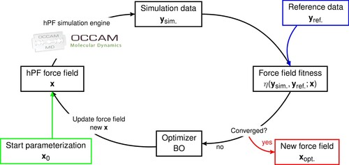
Figure 2. Summary of the hPF phospholipid model. Left: CG representation of the DPPC phospholipid and solvent. Right: Outline of the two terms in the hPF Hamiltonian.

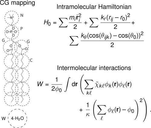
Figure 3. Density profiles and representative membrane snapshots from hPF-MD simulations of a DPPC bilayer using ${\tilde{\chi }}_{\mathrm{F}-\mathrm{H}}$ parameters [21] (left), particle-based simulations using the MARTINI CG force field (centre), and hPF-MD ${\tilde{\chi }}_{\mathrm{BO}}$ parameters (right). The table presents absolute deviations $S_k$ in the density profiles between the F-H and BO parameter simulations, and the reference MARTINI profile. Percentage deviations $S_{\mathrm{p}}$ are given in parenthesis. $S_k$ values are given in el./nm${}^3$.

Figure 4. Left: Feature importance as ranked by the mutual information measure between the fitness and the individual ${\tilde{\chi }}_{\mathrm{ij}}$ parameters, for hPF-MD simulations of a DPPC bilayer with randomly sampled $\tilde{\chi }$ matrices. Presented values are normalised relative to the most important parameter (${\tilde{\chi }}_{\mathrm{CW}}$) (arbitrary units). Inset details the low relative MI values found for the last six matrix elements (error bars omitted). $\tilde{\chi }$ parameters are included in order of decreasing feature importance (left). Right: Best fitness achieved (here using the average coefficient of determination, $R^2$, across all bead species) for each dimension of the parameter space subspace used in hPF-MD BO protocol runs on the DPPC bilayer system.

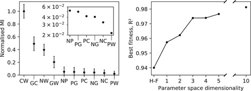
Figure 5. Top: Density profiles for hPF-MD DPPC bilayer simulations ran with Bayesian optimised parameter sets with four (left) and ten (right) included $\tilde{\chi }$ parameters. The four-parameter simulation uses ${\tilde{\chi }}_{\mathrm{F}-\mathrm{H}}$ values for all but the $\tilde{\chi }$ matrix elements with the highest feature importance, namely ${\tilde{\chi }}_{\mathrm{NW}}$, ${\tilde{\chi }}_{\mathrm{CW}}$, ${\tilde{\chi }}_{\mathrm{GW}}$, and ${\tilde{\chi }}_{\mathrm{GC}}$, c.f. column three of the table (bottom). Bottom: Resulting $\tilde{\chi }$ matrices from the BO protocol applied to hPF-MD simulations of a DPPC bilayer. Results reported for selected subspaces of the full 10-dimensional parameter space, with the ${\tilde{\chi }}_{\mathrm{ij}}$s shown in red being fixed and not part of the optimisation run. All $\tilde{\chi }$ values given in ${\mathrm{kJmol}}^{-1}$. Mean percentage errors, $S_{\mathrm{p}}$, associated with each set of optimised parameters is given in the last row.

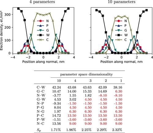
Table 1. Optimised $\tilde{\chi }$-matrix parameters found by the BO scheme for hPF-MD simulations of DPPC, DMPC, DSPC, and DOPC bilayer systems. The $\tilde{\chi }$ matrix elements are given in order of decreasing feature importance. Reference parameters are the Flory-Huggins (${\tilde{\chi }}_{\mathrm{F}-\mathrm{H}}$) parameters used in [21]. All values given in units of ${\mathrm{kJ}\mathrm{mol}}^{-1}$.

		Optimised with BO
	Ref [21]	DPPC	DMPC	DSPC	DOPC
C–W	33.75	42.24	41.20	40.15	35.00
G–C	6.30	10.47	13.78	14.65	14.61
N–W	−8.10	−3.77	−2.58	−3.02	−2.46
G–W	4.50	4.53	5.91	4.71	9.07
N–P	−1.50	−9.34	−4.34	−5.91	−3.40
P–G	4.50	8.04	5.26	7.25	8.45
N–G	6.30	1.97	3.37	2.99	4.92
P–C	13.50	14.72	19.72	16.16	12.52
P–W	−3.60	−1.51	−1.26	−2.17	−1.27
N–C	9.00	13.56	12.71	10.56	14.39

Table 2. Mean absolute deviations in electron density, $S_k$, with respect to the MARTINI reference density for the different lipids simulated with Bayesian optimised parameter sets on the different phospholipids (relative percentage deviations $S_{\mathrm{p}}$ in parenthesis). Comparison with data from De Nicola, using the baseline ${\tilde{\chi }}_{\mathrm{F}-\mathrm{H}}$ parameter set [21]. All $S_k$ values given $\mathrm{el}./{\mathrm{nm}}^3$.

	N	P	G	C	W	Average
DPPC
DPPC-optimised	4.65	4.10	6.52	7.26	8.91	6.29 (1.71%)
DMPC-optimised	4.45	4.05	6.44	8.37	8.36	6.34 (1.97%)
DOPC-optimised	5.39	8.15	12.05	9.81	6.51	8.38 (2.61%)
DSPC-optimised	5.02	6.08	8.71	9.40	9.63	7.76 (2.40%)
Reference [21]	9.29	12.19	20.51	12.23	12.82	13.41 (4.10%)
DMPC
DPPC-optimised	3.84	4.61	8.59	4.94	6.81	5.76 (1.85%)
DMPC-optimised	4.28	4.15	7.62	5.49	6.51	5.61 (1.81%)
DOPC-optimised	5.89	8.81	13.44	8.29	7.74	8.83 (2.87%)
DSPC-optimised	5.60	7.90	11.63	6.51	6.29	7.58 (2.45%)
Reference [21]	8.53	10.54	13.32	10.00	14.64	11.41 (3.63%)
DOPC
DPPC-optimised	3.28	4.55	6.27	7.59	8.55	6.05 (2.03%)
DMPC-optimised	3.77	3.61	5.44	8.87	7.22	6.78 (1.96%)
DOPC-optimised	3.21	3.37	5.11	8.41	8.63	5.74 (1.95%)
DSPC-optimised	3.21	2.98	5.25	8.80	10.58	6.16 (2.08%)
Reference [21]	10.33	6.21	13.38	13.98	24.26	13.63 (4.79%)
DSPC
DPPC-optimised	4.24	3.98	5.13	6.56	11.04	6.19 (1.86%)
DMPC-optimised	4.40	3.52	4.55	7.25	11.59	6.26 (1.88%)
DOPC-optimised	4.90	4.03	5.06	7.36	10.82	6.43 (1.94%)
DSPC-optimised	4.45	3.38	4.17	6.75	11.22	5.99 (1.80%)
Reference [21]	8.60	10.30	11.52	10.85	22.62	12.78 (3.80%)

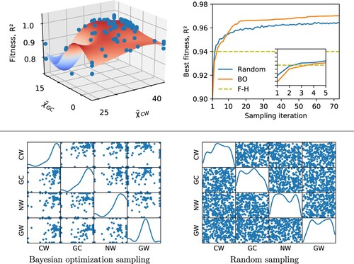
Figure 6. Top left: The surrogate objective fitness surface (here using the average coefficient of determination, $R^2$, across all bead species) in an example DPPC BO run with only the four parameters exhibiting the highest feature importance scores included (${\tilde{\chi }}_{\mathrm{CW}}$, ${\tilde{\chi }}_{\mathrm{GC}}$, ${\tilde{\chi }}_{\mathrm{NW}}$, and ${\tilde{\chi }}_{\mathrm{GW}}$). Individual samplings with their associated fitnesses are represented as blue dots. A projection onto the subspace spanned by ${\tilde{\chi }}_{\mathrm{CW}}$ and ${\tilde{\chi }}_{\mathrm{GC}}$ shown. All $\tilde{\chi }$ matrix elements are given in ${\mathrm{kJ}\mathrm{mol}}^{-1}$. Top right: Best DPPC simulation membrane fitness (average $R^2$) for BO and random sampling with only the four parameters exhibiting the highest feature importance scores included. Comparison with the fitness achieved by the reference ${\tilde{\chi }}_{\mathrm{F}-\mathrm{H}}$ parameter set. Inset details when BO and random sampling surpass the ${\tilde{\chi }}_{\mathrm{F}-\mathrm{H}}$ parameter set in terms of $R^2$ fitness. Bottom: Scatter matrices showing correlations between all pairs of $\tilde{\chi }$ parameters in a BO run on a DPPC bilayer (left) compared with random sampling (right). Only the four parameters exhibiting the highest feature importance scores are included in the sampling. The matrix diagonal shows the density of sampled points for each individual ${\tilde{\chi }}_{\mathrm{ij}}$ parameter. All $\tilde{\chi }$ matrix elements are given in ${\mathrm{kJ}\mathrm{mol}}^{-1}$.

A. De Nicola, Y. Zhao, T. Kawakatsu, D. Roccatano and G. Milano, J. Chem. Theory Comput. 7 (9), 2947–2962 (2011).

 PubMed Web of Science ®Google Scholar

Data availability statement

The data that support the findings of this study are available from the corresponding author upon reasonable request.