Figures & data
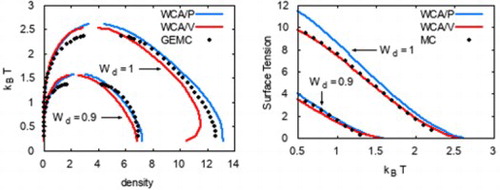
Figure 1. Model potential given by Equations (Equation1(1)
(1) ) and (Equation2
(2)
(2) ).
,
,
, and
.
![Figure 1. Model potential given by Equations (Equation1(1) ϕ(r)=ε[Wcw(r/Rc)−Wdw(r/Rd)],(1) ) and (Equation2(2) w(x)={1−6x2+6x3(x≤1/2)2(1−x)3(1/2<x≤1)0(x>1).(2) ). ϵ=18.75, Wc=2, Rc=0.8, and Rd=1.](/cms/asset/fbccf6ae-66a3-4be8-a4de-651379c7f24c/tmph_a_1802076_f0001_oc.jpg)
Figure 2. Density dependence of the difference in the radial distribution functions between HNC and MC for the system interacting with the reference () and the full (φ) potentials.
.
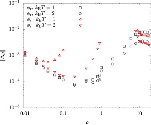
Figure 3. Pressure versus density isotherms. .
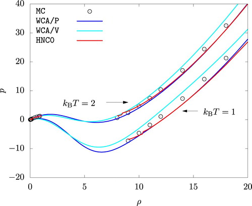
Figure 4. The radial distribution function from HNC and an MC simulation. To improve visibility, graphs for and 18 are shifted upwardly by 1 and 2, respectively.
and
.
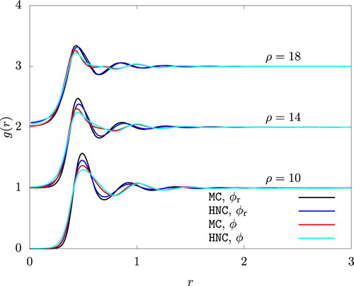
Figure 5. The relative importance in the thermodynamic perturbation theory of the second order term in comparison to the first order term
given by Equations (Equation27
(27)
(27) ) and (Equation12
(12)
(12) ), respectively.
.
![Figure 5. The relative importance in the thermodynamic perturbation theory of the second order term ψa(2) in comparison to the first order term ψa given by Equations (Equation27(27) ψa(2)(T,ρ)≈−14βρ(∂pref∂ρ)T−1∫[ϕa(r)]2gr(r)dr,(27) ) and (Equation12(12) ψa(T,ρ)=12βρ∫ϕa(r)gr(r)dr.(12) ), respectively. Wd=1.](/cms/asset/6a1dc170-35d8-4c55-8a31-583aff1b684d/tmph_a_1802076_f0005_oc.jpg)
Figure 6. Phase diagram showing vapour-liquid phase coexistence.
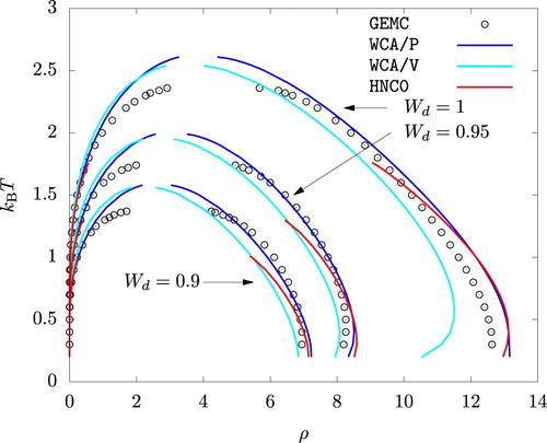
Figure 7. Vapor phase density at saturation.
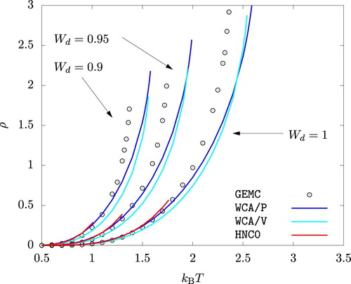
Figure 8. Temperature dependence of the the liquid phase density at p = 0.01, p = 1, and p = 10. . For each method and at each temperature, the density is larger for a higher pressure.
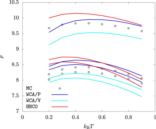
Figure 9. Surface tension γ of the vapour-liquid interface at saturation.
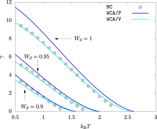
Figure 10. The density , beyond which a high density fluid phase is mechanically unstable, plotted versus temperature. An open symbol indicates a fluid phase with a negative pressure.
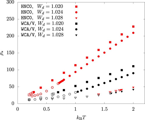
Figure 11. Liquid phase density at saturation () shown with the onset of mechanical instability (
) and the maximum density (
) above which iterative solution of Equations (Equation7
(7)
(7) ) and (Equation8
(8)
(8) ) fails.
. An open symbol for
indicates a negative pressure.
![Figure 11. Liquid phase density at saturation (ρleq) shown with the onset of mechanical instability (ρ⋆) and the maximum density (ρmax) above which iterative solution of Equations (Equation7(7) hr(r)=cr(r)+ρ∫cr(|r−r′|)hr(r′)dr′(7) ) and (Equation8(8) cr(r)=hr(r)−ln[hr(r)+1]−βϕr(r),(8) ) fails. Wd=1.024. An open symbol for ρ⋆ indicates a negative pressure.](/cms/asset/37230cbf-e1d3-4156-aba1-4bbef0bb54cd/tmph_a_1802076_f0011_oc.jpg)
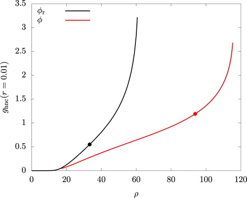
Figure 12. Density dependence of the radial distribution function at r = 0.01 using the HNC closure. and
. The filled circules indicate the values at the onset of mechanical instability (
).