A new boundary driven NEMD scheme for heat and particle diffusion in binary mixtures

Figures & data

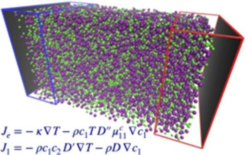
Figure 1. (a) The subdivision of the simulation box into the different regions, the inner zone, white background, is where the fields and currents are measured, while the regions where the thermostats act on particle velocities are highlighted by different shades of blue for the lower temperature $T_C$, on the left, and red for the higher temperature $T_H$, on the right, with particle exchanges taking place in the darker zones to fix the concentrations to the values $x_{1C}$ and $x_{1H}$, respectively, as described in the text. Periodic boundary conditions are only applied in the x, y-directions, while in the z-direction the system is confined by repulsive walls, dark grey area, placed at the edges of the box. (b) A snapshot is rendered with VMD [14] from the simulation data with temperature gradient $\mathrm{\nabla }T>0$ and molar fraction gradient $\mathrm{\nabla }{x}_1>0$ between the two reservoirs along the z-axis (blue arrow on-axis compass). Note a separation of Kr species (larger size, purple) particles gathering in the higher temperature region, $T_H$, as a result of the imposed concentration gradient. The empty spaces in the z-direction are the regions rarely explored by the particles where the wall potential is highly repulsive.

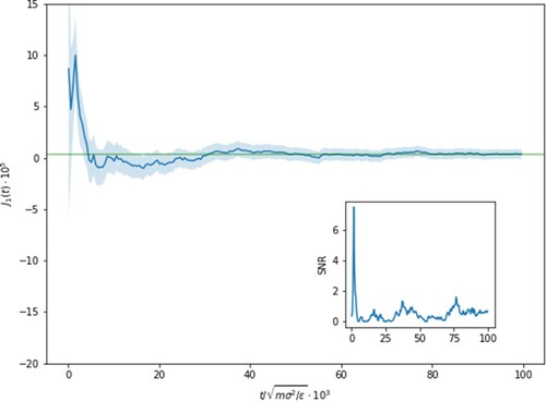
Figure 2. Running average of the mass flux for $(\mathrm{\Delta }T,\mathrm{\Delta }{x}_1)=(0.1,0.1)$ with error shown by the shaded region. Relaxation to the stationary value occurs after $t=30\times {10}^3$ units with minor long-living fluctuations around the mean value afterwards as shown by the horizontal green line. Shown in the inset is the signal-to-noise ($\frac{{\mu }^2}{{\sigma }^2}$) ratio which encouragingly continues to steadily climb with increasing statistics.

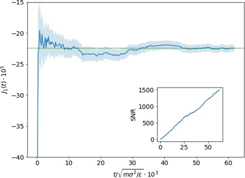
Figure 3. A plot of the temperature (a), mol fraction (b), mass flux of Kr (c), and energy flux (d) as a function of position along the z-direction measured in units of slice width, i.e. ${\sigma }_{\mathrm{Kr}}$, with $(\mathrm{\Delta }T,\mathrm{\Delta }{x}_1)=(0.1,-0.045)$. Each point represents the average over a slice and $T_H/T_C$ are indicated by the red(right)/blue(left) shaded regions. The reservoir region in which the mol fraction is controlled consists of only the first and last 3 slices in $T_H/T_C$ as described in the text and are shaded darker. The values reported in (c) and (d) are for the flux averaged across the entire bulk region, neglecting the slices in direct contact with the thermostats and where the faint green line shows the zero level. The vertical green lines in panels (a) and (b) show the equidistant point in the bulk from the reservoirs and it may be observed that the concentration profile (b) is not symmetric in shape for the two species across the bulk and indicates a preference of the heavier Kr towards the colder regions.

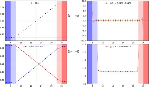
Figure 4. The estimated standard deviation for $J_1$ from the block analysis of three independent trajectory segments each of ${10}^7$ timesteps for the ($\mathrm{\Delta }T=0.1,\mathrm{\Delta }{x}_1=0$) condition. Values for ($\sqrt{s_{{\tau }_b}^2/N_b}$) are plotted against the number of timesteps in each block ${\tau }_b$, where $N_b$ is the number of blocks and $N_b{\tau }_b={10}^7$. The region between 100 and 10,000 steps shows a relatively flat profile, which implies that there the block averages can be considered as independent samples. Going to shorter intervals of time, the decrease can be traced back to increasing correlations while at the other end the number of blocks $N_b$ becomes too small to provide a reliable estimate of the variance of the sample.

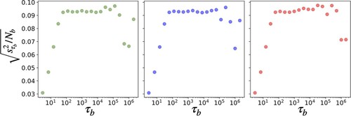
Table 1. Check of linearity using the measured values of the temperature gradient, the energy flux, the molar fraction gradient and the mass flux for component 1, reported in LJ units.

	${10}^3\cdot \mathrm{\nabla }T$	${10}^3\cdot {\mathbf{J}}_e$	${10}^3\cdot \mathrm{\nabla }{x}_1$	${10}^5\cdot {\mathbf{J}}_1$
(a)	1.861 (0.004)	−8.50 (0.03)	−0.121 (0.004)	−3.56 (0.25)
(b)	0.003 (0.004)	0.07 (0.03)	1.540 (0.004)	−7.73 (0.25)
(sum)	1.864 (0.006)	−8.32 (0.4)	1.419 (0.006)	−11.29 (0.35)
(a+b)	1.853 (0.004)	−8.39 (0.03)	1.395 (0.004)	−10.73 (0.25)
(rel.err)	0.6	0.8	1.7	5

The value obtained summing the fluxes for case (a) and case (b) are compared with the values measured with the case (a+b) with boundary values chosen to impose simultaneously both the temperature and the molar fraction gradients imposed in (a) and (b) separately. The fluxes satisfy the linear regime hypothesis within the numerical accuracy, with the resulting gradients adding up consistently. The relative error $\frac{(\mathrm{a}+\mathrm{b})-(\mathrm{sum})}{(\mathrm{sum})}$ is also included. Note that, since we can impose the boundary values but not the gradients, the check cannot be performed with exactly the same total gradients.

Figure 5. The temperature (top) and concentration (bottom) profiles where panels (a), (b) and (c) are for conditions $\mathrm{\Delta }T,\mathrm{\Delta }{x}_1=\{(0.1,0.1),(0.1,0),(0,0.1)\},$ respectively. Each point represents the average over a slice and regions $T_H/T_C$ are indicated by the red(right)/blue(left) shaded areas. The reservoir region in which the mol fraction is controlled consists of only the first and last 3 slices in $T_H/T_C$ as described in the text and are shaded darker. From (b), one can see that while the concentration is equal at both edges, it is not enough to force the profile in the bulk to be uniform and a small gradient emerges, with opposite sign to the temperature gradient.

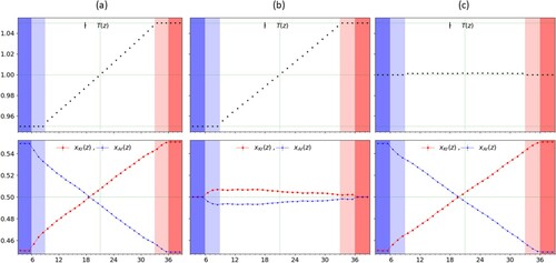
Table 2. Heat and mass transport coefficients from the BD-NEMD protocol.

$D$	$D^{\mathrm{\prime }}$	$\kappa$	${\mu }_{11}$	$S_T=D^{\mathrm{\prime }}/D$
0.0501 (0.001)	0.087 (0.003)	4.603 (0.009)	−0.83 (0.34)	1.7 (0.1)

All values reported are in LJ units with error given in the parenthesis.

Table 3. Comparison of the Onsager coefficients between our results (BD-NEMD) and those from the mechanical perturbation scheme by Sarman and Evans [2] for a system of 1024 particles of Ar-Kr.

Onsager coefficient	BD-NEMD ($T=1.0,n=0.725$)	Ref. [2] ($T=0.965,n=0.7137$)
$L_{qq}$	4.60 (0.01)	4.24 (0.01)
$L_{1q}$	0.0214 (0.0007)	0.0182 (0.001)
$L_{11}$	0.0191 (0.0075)	0.0174 (0.0005)

Table 4. Results of the measured fluxes and gradients in the bulk for the experimentally inspired protocol where $J_1\approx 0$.

Condition	${10}^5\times J_1$	${10}^3\times J_e$	${10}^3\times \mathrm{\nabla }T$	${10}^3\times \mathrm{\nabla }{x}_1$	$S_T$
Natural	−0.2 (0.3)	−16.85 (0.03)	3.678 (0.004)	−1.512 (0.004)	1.69 (0.07)
Driven	+0.2 (0.1)	−16.89 (0.02)	3.691 (0.002)	−1.612 (0.002)	1.70 (0.04)

The results dubbed Driven were obtained imposing $\mathrm{\Delta }T=0.1$ and $\mathrm{\Delta }{x}_1=-0.045$, fixing both the thermal and molar fraction gradients, while Natural refers to values with only $\mathrm{\Delta }T=0.1$ imposed, fixing the temperature gradient and allowing the system to relax naturally until mass equilibrium is reached and a stationary concentration gradient is created.

Figure 6. Running average of the mass flux with the shaded region showcasing the error with $\mathrm{\Delta }T=0.1$ and $\mathrm{\Delta }{x}_1=-0.045$ to achieve mass equilibrium. Note that even after $t=40\times {10}^3$, there is still a measurable mass flux value and that at $t=100\times {10}^3$ the uncertainty is as large as the signal. This is shown more prominently in the inset where the signal-to-noise is given over time and contrasting to the inset of Figure 2 where the SNR rose monotonically with simulation time.

W. Humphrey, A. Dalke and K. Schulten, J. Mol. Graph. 14, 33–38 (1996). doi:https://doi.org/10.1016/0263-7855(96)00018-5

 PubMed Web of Science ®Google Scholar

S. Sarman and D.J. Evans, Phys. Rev. A 45 (4), 2370–2379 (1992). doi:https://doi.org/10.1103/PhysRevA.45.2370

 PubMed Web of Science ®Google Scholar