Figures & data

Figure 1. (a) Schematic of the key parameters and
used to characterise halogen–halogen contacts. If
the contact is type I and not considered halogen bonded. Type II contacts typically exhibit
and
. For an ideal halogen bond
and
. (b) Schematic of the X
motif, which consists of three type II contacts in a trigonal geometry.
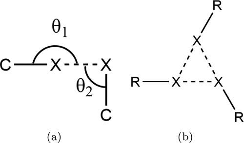
Figure 2. (a) Chemical structure of triiodomesitylene, the first species shown to exhibit the X halogen bonding motif. (b) Chemical structure of 1,3,5-triiodo-2,4,6-trifluorobenzene, the species considered in this work. Despite the structural similarity the fluorinated compound was found not to exhibit the X
bonding motif in the bulk [Citation38].
![Figure 2. (a) Chemical structure of triiodomesitylene, the first species shown to exhibit the X3 halogen bonding motif. (b) Chemical structure of 1,3,5-triiodo-2,4,6-trifluorobenzene, the species considered in this work. Despite the structural similarity the fluorinated compound was found not to exhibit the X3 bonding motif in the bulk [Citation38].](/cms/asset/1ace6472-a5a9-40c8-9cb8-1d0558e46ec9/tmph_a_1900940_f0002_ob.jpg)
Figure 3. Collected diffractogram of papyex dosed with TITFB, the Graphite 002 peak is labelled. Below 5 small-angle scattering is significant. In addition to the bulk graphite peak several additional ”sawtooth” peaks of much lower intensity can be seen.
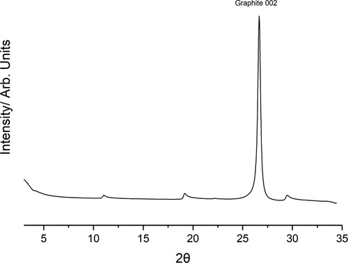
Figure 4. Comparison between the collected (black) and modelled (blue) diffraction pattern for the TITFB monolayer structure shown in (a), (a) Optimised experimental structure for the TITFB monolayer. The unit mesh is hexagonal with lattice parameters Å
. (b) Background subtraction of the monolayer pattern (black) compared to the modelled pattern (blue).
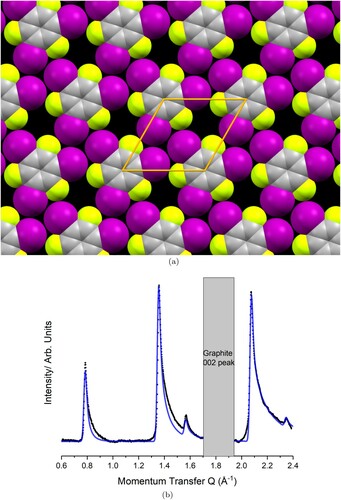
Table 1. Key geometric parameters for several relevant systems. and
are defined in Figure (a).
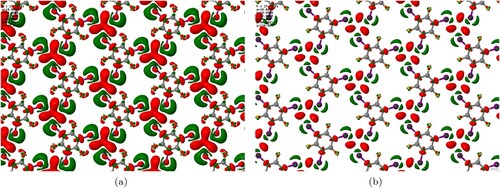
Figure 5. Maps of electron density accumulation (red) and depletion (green) for the condensed TITFB monolayer, relative to the electron density of isolated molecules constrained to the same local geometries but with doubled lateral lattice constant. Isosurface thresholds are set at (a) electrons.Å
and (b)
electrons.Å
.