
Figures & data
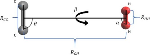
Figure 1. Definition of the body-fixed coordinates system.
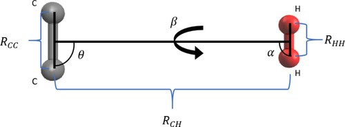
Figure 2. Cuts of C/H
PES along the radial coordinate
for the three H
orientations used in the present calculations, plus its average value. Different different values of θ are shown.
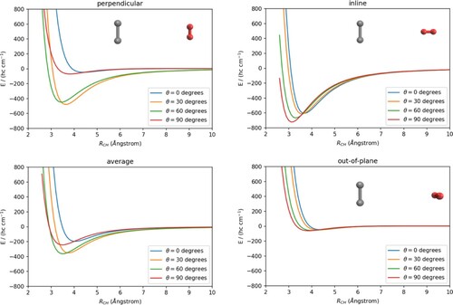
Figure 3. Contour plots of C-H
averaged 2D-PES (left) and full 2D-PES for the C
-Ar(right).The levels of energy contours are given in units of (hc cm
).
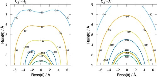
Figure 4. Radial coefficients of the expansion given by Equation (Equation2(2)
(2) ) for C
interacting with H
(solid lines) and Ar (dashed lines). Only the first three, most important radial functions are shown.
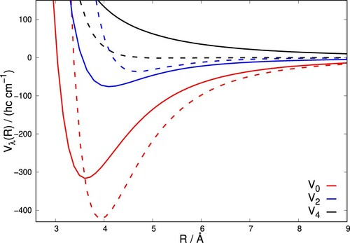
Figure 5. Rotationally inelastic scattering cross-sections for C colliding with p-H
($j= 0$) (solid lines) and He (dashed lines) for excitation (top panels) and quenching (bottom panels).
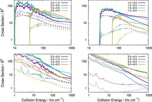
Figure 6. Rotationally inelastic scattering cross-sections for pseudo-singlet C colliding with para-H
(j = 0) (solid lines) and with Ar (dashed lines) for excitation (top panels) and quenching (bottom panels).
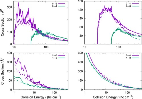
Figure 7. Examples of rotationally inelastic rate constants for for C
colliding with H
and He. Rate constants obtained by multiplying those of He by
and
factors are also shown.
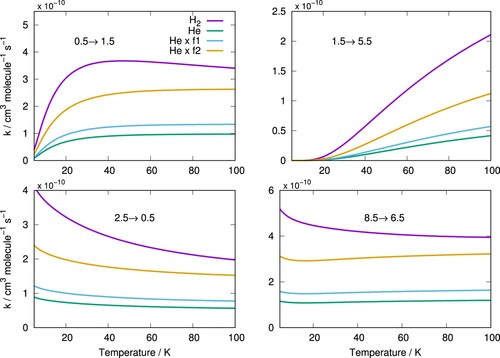
Figure 8. Rotationally inelastic rate constants for corresponding transitions of Figure for C
colliding with p-H
(j = 0) (solid lines) and Ar (dashed lines).
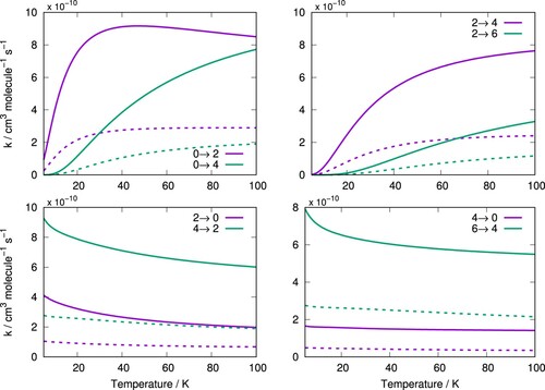
Figure 9. Computed quenching functions for C interacting with p-H
(j = 0) (solid lines) and He (dashed lines) as function of the expected range of trap temperatures. Two different initial rotational states are shown as examples for both systems. See main text for further comments.
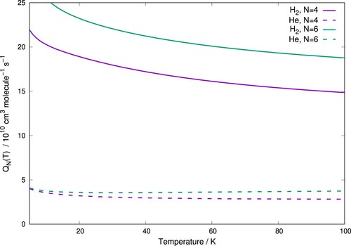
Figure 10. Thermalisation of C rotational N states during collisions with He, Ar and H
at 20 K. Initial populations are taken from a Boltzmann distribution at 100 K. Gas pressure η is set as
cm
except for the ‘low P’ plot where
cm
was used. Vertical dashed line indicates when populations reach steady-state value as defined in the main text.
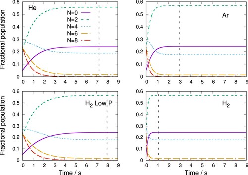
Figure 11. Thermalisation of C rotational states during collisions with He, Ar and p-H
(j = 0) (right panel) at 60 K Other parameters are the same as those of Figure .
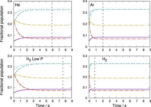
Table 1. Quadrupole transitions probabilities for transitions for C
and para-H
[Citation71]. Units of s
.