An excited state coupled-cluster study on indigo dyes

Figures & data

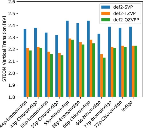
Figure 1. Vertical transition energies computed by the DLPNO-STEOM method for a set of symmetrically substituted indigo dyes. Data plotted from Table 2.

Scheme 1. Simplified central ‘H chromophore’ of indigo.

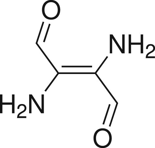
Table 1. Total energies for the ${\mathrm{S}}_0$ and ${\mathrm{S}}_1$ states of the H chromophore $({\text{E}}_{\mathrm{h}})$. The excitation energy to the S₁ state, ω, is computed in eV. Here, we understand ‘STEOM’ to mean ‘DLPNO-STEOM’ with identical settings as in the remaining calculations in this paper. All other methods are canonical.

	CASSCF	fic-NEVPT2	uc-MRCI	fic-MRCC	EOMCC	STEOM
S${}_0$	−413.304138	−414.457377	−414.457254	−414.507567	−414.492813	−414.492887
S${}_1$	−413.129797	−414.346606	−414.341664	−414.379725	−414.368914	−414.381096
ω	4.744	3.014	3.145	3.479	3.371	3.042

Table 2. Vertical transition energies computed by the DLPNO-STEOM method for a set of symmetrically substituted indigo dyes.

Compound	def2-SVP	def2-TZVP	def2-QZVPP
Indigo	2.39	2.23	2.23
4,4'-Bromoindigo	2.37	2.21	2.19
4,4'-Chloroindigo	2.38	2.22	2.21
5,5'-Bromoindigo	2.34	2.18	2.16
5,5'-Chloroindigo	2.32	2.17	2.15
5,5'-Nitroindigo	2.44	2.29	2.28
6,6'-Bromoindigo	2.42	2.26	2.24
6,6'-Chloroindigo	2.44	2.28	2.25
6,6'-Nitroindigo	2.33	2.16	2.13
7,7'-Bromoindigo	2.39	2.22	2.21
7,7'-Chloroindigo	2.38	2.23	2.22
Deviation from def2-QZVPP
Max(−)	0.16	0.00
ME	0.17	0.01
Max(+)	0.19	0.03
SD	0.01	0.01
MAE	0.17	0.01

All values are given in eV.

Table 3. Solvation effects compared to gas-phase STEOM calculations. Solvents sorted with increasing dielectric constant ε from left to right.

	CCl4	Xylene	Benzene	CHCl3	TCE	EtOH	DMSO
ε	2.24	2.27	2.28	4.9	8.2	24.3	47.2
Indigo	−0.099	−0.101	−0.101	−0.137	−0.153	−0.155	−0.164
4,4'-Bromoindigo	−0.100	−0.102	−0.102	−0.137	−0.156	−0.165	−0.173
4,4'-Chloroindigo	−0.102	−0.104	−0.104	−0.140	−0.155	−0.166	−0.175
5,5'-Bromoindigo	−0.093	−0.095	−0.095	−0.124	−0.138	−0.145	−0.153
5,5'-Chloroindigo	−0.096	−0.097	−0.098	−0.121	−0.135	−0.142	−0.150
5,5'-Nitroindigo	−0.082	−0.083	−0.075	−0.109	−0.123	−0.128	−0.138
6,6'-Bromoindigo	−0.100	−0.102	−0.103	−0.135	−0.151	−0.156	−0.168
6,6'-Chloroindigo	−0.102	−0.104	−0.104	−0.138	−0.153	−0.162	−0.170
6,6'-Nitroindigo	−0.106	−0.127	−0.127	−0.157	−0.175	−0.185	−0.195
7,7'-Bromoindigo	−0.078	−0.080	−0.081	−0.108	−0.120	−0.126	−0.134
7,7'-Chloroindigo	−0.087	−0.089	−0.089	−0.116	−0.132	−0.134	−0.142
Average	−0.095	−0.099	−0.098	−0.129	−0.145	−0.151	−0.160

All values are given in eV.

Table 4. Benchmark results: the CPCM-corrected DLPNO-STEOM excitation energy (ω), the VG correction ${\omega }_{\mathrm{VG}}$, the 0–0 transition energy (${\omega }_{0-0}$), the experimental absorption band maxima (${\omega }_{\exp }$) [13] and the error of the total STEOM estimate with respect to experiment ($\mathrm{\Delta }\omega$).

Name	Solvent	ω	${\omega }_{\mathrm{VG}}$	${\omega }_{0-0}$	${\omega }_{exp}$	$\mathrm{\Delta }\omega$
Indigo	Benzene	2.13	−0.05	2.09	2.08	0.00
Indigo	CCl${}_4$	2.13	−0.05	2.09	2.09	0.00
Indigo	CHCl${}_3$	2.10	−0.05	2.05	2.05	0.00
Indigo	DMSO	2.07	−0.05	2.02	2.00	0.02
Indigo	EtOH	2.08	−0.05	2.03	2.04	−0.01
Indigo	TCE	2.08	−0.05	2.03	2.02	0.01
4-Bromoindigo	TCE	2.08	−0.05	2.03	2.03	−0.01
5-Bromoindigo	Benzene	2.12	−0.05	2.07	2.05	0.02
5-Bromoindigo	TCE	2.07	−0.05	2.02	2.02	0.00
6-Bromoindigo	TCE	2.08	−0.05	2.03	2.06	−0.03
7-Bromoindigo	TCE	2.08	−0.05	2.03	2.05	−0.02
4,4'-Bromoindigo	TCE	2.06	−0.05	2.00	2.03	−0.02
4,4'-Chloroindigo	CHCl${}_3$	2.08	−0.05	2.03	2.05	−0.02
4,4'-Chloroindigo	EtOH	2.06	−0.05	2.00	2.03	−0.02
4,4'-Chloroindigo	TCE	2.07	−0.05	2.01	2.02	−0.01
4,4'-Chloroindigo	Xylene	2.12	−0.05	2.07	2.07	0.00
4,4'-Methoxycarbonylindigo	EtOH	2.03	−0.05	1.98	2.03	−0.04
4,4'-Methoxyindigo	TCE	2.09	−0.06	2.03	2.06	−0.02
5,5'-Bromoindigo	CHCl${}_3$	2.06	−0.05	2.00	2.03	−0.03
5,5'-Bromoindigo	EtOH	2.03	−0.05	1.98	2.01	−0.03
5,5'-Bromoindigo	TCE	2.04	−0.05	1.99	2.00	−0.01
5,5'-Bromoindigo	Xylene	2.08	−0.05	2.03	2.05	−0.02
5,5'-Chloroindigo	EtOH	2.02	−0.05	1.97	2.02	−0.04
5,5'-Chloroindigo	TCE	2.03	−0.05	1.98	2.00	−0.02
5,5'-Chloroindigo	Xylene	2.07	−0.05	2.02	2.05	−0.03
5,5'-Fluoroindigo	CHCl${}_3$	2.02	−0.05	1.97	2.01	−0.04
5,5'-Fluoroindigo	TCE	2.01	−0.05	1.96	2.02	−0.06
5,5'-Methoxyindigo	TCE	1.90	−0.07	1.83	1.91	−0.08
5,5'-Methylindigo	CHCl${}_3$	2.04	−0.05	1.99	2.01	−0.02
5,5'-Methylindigo	TCE	2.03	−0.05	1.97	2.00	−0.03
5,5'-Nitroindigo	TCE	2.16	−0.05	2.11	2.14	−0.03
6,6'-Bromoindigo	TCE	2.11	−0.05	2.06	2.11	−0.05
6,6'-Bromoindigo	Xylene	2.16	−0.04	2.11	2.10	0.01
6,6'-Chloroindigo	EtOH	2.12	−0.05	2.07	2.18	−0.11
6,6'-Chloroindigo	TCE	2.13	−0.05	2.08	2.10	−0.02
6,6'-Chloroindigo	Xylene	2.18	−0.04	2.13	2.22	−0.08
6,6'-Fluoroindigo	TCE	2.20	−0.05	2.14	2.18	−0.03
6,6'-Methoxyindigo	TCE	2.24	−0.06	2.18	2.16	0.02
6,6'-Methylindigo	TCE	2.11	−0.05	2.06	2.08	−0.02
6,6'-Methylindigo	Xylene	2.15	−0.05	2.10	2.11	−0.01
6,6'-Nitroindigo	TCE	1.98	−0.05	1.93	1.95	−0.02
6,6'-Nitroindigo	Xylene	2.03	−0.04	1.99	1.96	0.03
7,7'-Bromoindigo	TCE	2.10	−0.06	2.05	2.05	0.00
7,7'-Chloroindigo	EtOH	2.09	−0.06	2.04	2.10	−0.07
7,7'-Chloroindigo	TCE	2.09	−0.06	2.04	2.06	−0.02
7,7'-Fluoroindigo	CHCl${}_3$	2.09	−0.05	2.04	2.00	0.03
7,7'-Fluoroindigo	TCE	2.08	−0.06	2.02	2.05	−0.03
7,7'-Methoxyindigo	TCE	1.97	−0.08	1.89	1.93	−0.03
7,7'-Methylindigo	CHCl${}_3$	2.08	−0.06	2.02	2.03	−0.01
7,7'-Methylindigo	Xylene	2.11	−0.06	2.06	2.05	0.00
5,5',7-Bromoindigo	Xylene	2.09	−0.05	2.04	2.03	0.01
4,4',5,5'-Bromoindigo	Benzene	2.07	−0.05	2.02	2.02	0.00
4,4',5,5'-Chloroindigo	TCE	2.03	−0.05	1.98	1.99	−0.01
4,4',6,6'-Chloroindigo	TCE	2.09	−0.05	2.04	2.08	−0.04
4,4',6,6'-Methylindigo	Xylene	2.13	−0.05	2.08	2.09	0.00
4,4',7,7'-Chloroindigo	TCE	2.06	−0.06	2.01	2.03	−0.03
4,4',7,7'-Chloroindigo	Xylene	2.11	–0.05	2.05	2.08	−0.02
4,4',7,7'-Methylindigo	Xylene	2.07	−0.06	2.01	2.06	−0.05
5,5',6,6'-Chloroindigo	TCE	2.05	−0.05	2.00	2.05	−0.05
5,5',6,6'-Methylindigo	Xylene	2.10	−0.05	2.04	2.05	−0.01
5,5',7,7'-Bromoindigo	Benzene	2.08	−0.06	2.03	2.02	0.01
5,5',7,7'-Bromoindigo	CHCl${}_3$	2.06	−0.06	2.00	2.02	−0.01
5,5',7,7'-Bromoindigo	EtOH	2.04	−0.06	1.98	2.00	−0.02
5,5',7,7'-Bromoindigo	TCE	2.05	−0.06	1.99	2.00	0.00
5,5',7,7'-Bromoindigo	Xylene	2.08	−0.06	2.03	2.02	0.00
5,5',7,7'-Chloroindigo	EtOH	2.03	−0.06	1.97	2.02	−0.04
5,5',7,7'-Chloroindigo	TCE	2.04	−0.06	1.98	2.00	−0.02
5,5',7,7'-Chloroindigo	Xylene	2.07	−0.06	2.01	2.03	−0.02
6,6',7,7'-Chloroindigo	TCE	2.12	−0.05	2.07	2.10	−0.03
6,6',7,7'-Methylindigo	Xylene	2.08	−0.05	2.03	2.08	−0.06
4,4'-Chloro-5,5'-bromoindigo	CHCl${}_3$	2.04	−0.05	1.99	2.03	−0.04
4,4'-Chloro-5,5'-bromoindigo	TCE	2.02	−0.05	1.97	2.00	−0.03
4,4'-Chloro-5,5'-bromoindigo	Xylene	2.07	−0.05	2.02	2.02	0.00
5,5'-Chloro-7,7'-bromoindigo	Xylene	2.07	−0.06	2.02	2.03	−0.01
4,4',5,5',6,6'-Chloroindigo	TCE	2.03	−0.05	1.98	2.03	−0.05
4,4',5,5',7,7'-Bromoindigo	CHCl${}_3$	2.03	−0.06	1.98	1.99	−0.01
4,4',5,5',7,7'-Bromoindigo	Xylene	2.05	−0.05	1.99	2.01	−0.02
4,4',5,5',7,7'-Chloroindigo	TCE	2.03	−0.06	1.98	2.02	−0.04
4,4',5,5',7,7'-Chloroindigo	Xylene	2.07	−0.05	2.02	2.02	−0.01
4,4',6,6',7,7'-Chloroindigo	TCE	2.09	−0.05	2.03	2.08	−0.05
5,5',6,6',7,7'-Chloroindigo	TCE	2.05	−0.05	2.00	2.07	−0.07
5,5',7,7'-Bromo-6,6'-aminoindigo	Xylene	2.31	−0.07	2.25	2.22	0.03
4,4',5,5',6,6',7,7'-Chloroindigo	EtOH	2.03	−0.05	1.98	2.05	−0.07
4,4',5,5',6,6',7,7'-Chloroindigo	TCE	2.04	−0.05	1.98	2.02	−0.04
4,4',5,5',6,6',7,7'-Chloroindigo	Xylene	2.06	−0.05	2.01	2.04	−0.03

All values reported in eV.

Table 5. Statistical evaluation of the VG corrections (${\omega }_{\mathrm{VG}}$) and the errors in DLPNO-STEOM 0–0 transition energies (${\omega }_{0-0}$) from Table 4 with respect to the experimental values (eV).

	${{\omega }_{\mathrm{VG}}}^{†}$	${\omega }_{0-0}$
Max(−)	−0.08	−0.11
ME	−0.05	−0.02
Max(+)	−0.04	0.03
SD	0.01	0.03
MAE	0.05	0.03

${}^{†}$ For ${\omega }_{\mathrm{VG}}$, the smallest, average, maximum, … shifts are reported instead of errors.

Figure 2. Normalized error density distribution with respect to experiment, $\mathrm{\Delta }\omega$, from Table 4, with a Gaussian probability density function overlaid.

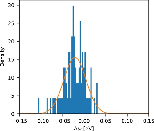
Figure 3. The effect of chemical substitutions on excitation energies. The dashed line indicates perfect agreement between theory and experiment, the shaded zone signifies the region within which the agreement is within ±0.1 eV.

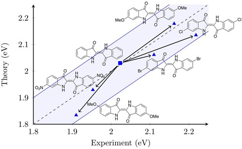
Figure 4. Normalized VIS absorption spectra for indigo, 6-bromoindigo, and 6,6'-dibromoindigo in DMSO. The unshifted computed spectra are presented with an inhomogeneous line width of $700{\mathrm{cm}}^{-1}$ as well as sticks for each vibrational mode. The experimental spectra were obtained from Ref. [83].

Figure 5. The spectrum of Tyrian purple and the 0–0 transition energies of three of its components studied in this paper. The shaded area corresponds to the region where indirubin dyes absorb (its width chosen from the spread between the band maxima of indigorubin dyes in Ref. [83] with an additional $500{\mathrm{cm}}^{-1}$ in both directions).

D. Jacquemin, J. Preat, V. Wathelet and E.A. Perpète, J. Chem. Phys. 124 (7), 074104 (2006). doi:10.1063/1.2166018

 PubMedGoogle Scholar

Z.C. Koren, in Indirubin, the Red Shade of Indigo, edited by L. Meijer, N. Guyard, L. Skalsounis and G. Eisenbrand, Chap. 5 (Ed. ‘Life in Progress’, Roscoff, France, 2006).

 Google Scholar