Calculation of reaction rate constants from a classical Wigner model based on a Feynman path integral open polymer

Figures & data

Figure 1. $C_{\text{fs}}\left(t\right)$ for an Eckart potential with $\text{β}\hslash \omega =1$. The traces are calculated with the y-version of OPCW for different N, exact Classical Mechanics (CM), exact Classical Wigner (CW), and exact Quantum Mechanics (QM). The QM-line only shows the result in the long time limit (not the time dependent function). The numbers in parenthesis are the number of Monte Carlo steps used. The top and bottom lines of each type show the standard deviation of the results (but uncertainties are often so small that the lines are not clearly distinguished).

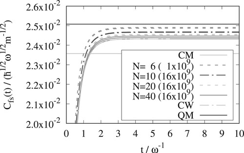
Figure 2. As in Figure 1 but for the x-version of OPCW.

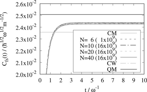
Figure 3. As in Figure 1 but for $\text{β}\hslash \omega =3$.

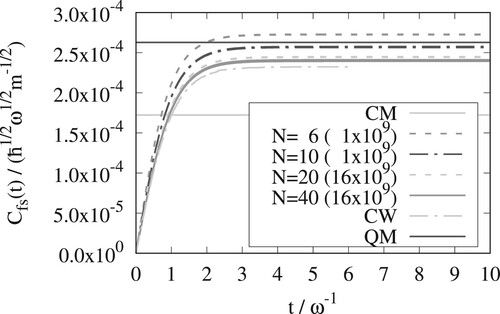
Figure 4. As in Figure 1 but for $\text{β}\hslash \omega =3$ and the x-version of OPCW.

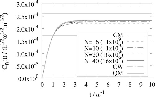
Figure 5. As in figure 1 but for $\text{β}\hslash \omega =6$.

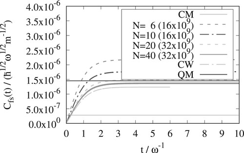
Figure 6. As in figure 1 but for $\text{β}\hslash \omega =6$ and the x-version of OPCW.

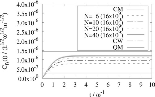
Figure 7. As in figure 1 but for $\text{β}\hslash \omega =12$ and the x-version of OPCW.

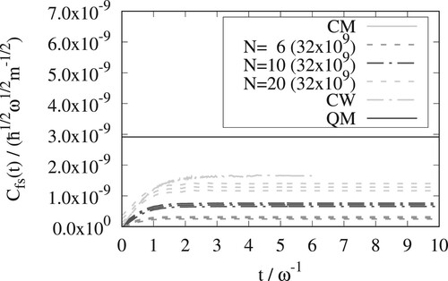
Table 1. Rate constants ($k_{\text{r}}$) for different inverse temperatures (β) for the Eckart barrier described in Equation 24(24) $V_{\text{Eckart}}\left(x\right)=\frac{6\hslash \omega }{\pi }{\mathrm{s}\mathrm{e}\mathrm{c}\mathrm{h}}^2\left(\sqrt{\frac{\pi m\omega }{12\hslash }}x\right),$(24) . Comparision of OPCW[x-version, N = 40], Ring Polymer Molecular Dynamics (RPMD), classical mechanics (CM), exact Classical Wigner (CW), and quantum mechanics (QM). Note that for $\text{β}=12$ only N = 20 was used for OPCW.

	$k_{\text{r}}/\left({\hslash }^{\frac{1}{2}}{\omega }^{\frac{1}{2}}{m}^{-\frac{1}{2}}\right)$
$\text{β}\hslash \omega$	OPCW	RPMD	CM	CW	QM
1	$6.10\times {10}^{-2}$	$6.17\times {10}^{-2}$	$5.9084\times {10}^{-2}$	$6.10\times {10}^{-2}$	$6.2856\times {10}^{-2}$
3	1.01 $\times {10}^{-3}$	1.07 $\times {10}^{-3}$	7.4821 $\times {10}^{-4}$	1.01 $\times {10}^{-3}$	1.1409 $\times {10}^{-3}$
6	7.39 $\times {10}^{-6}$	7.46 $\times {10}^{-6}$	1.7186 $\times {10}^{-6}$	7.61 $\times {10}^{-6}$	8.9347 $\times {10}^{-6}$
12	$1.\times {10}^{-8}$	1.39 $\times {10}^{-8}$	1.2824 $\times {10}^{-11}$	1.4 $\times {10}^{-8}$	2.5306 $\times {10}^{-8}$

Table 2. Tunneling factors (Γ) for different inverse temperatures (β) for the Eckart barrier described in Equation 24(24) $V_{\text{Eckart}}\left(x\right)=\frac{6\hslash \omega }{\pi }{\mathrm{s}\mathrm{e}\mathrm{c}\mathrm{h}}^2\left(\sqrt{\frac{\pi m\omega }{12\hslash }}x\right),$(24) . Comparision of OPCW[x-version, N = 40], Ring Polymer Molecular Dynamics (RPMD), exact Classical Wigner (CW), and exact results. Note that for $\text{β}=12$ only N = 20 was used for OPCW.

$\text{β}\hslash \omega$	${\mathrm{\Gamma }}_{\text{OPCW}}$	${\mathrm{\Gamma }}_{\text{RPMD}}$	${\mathrm{\Gamma }}_{\text{CW}}$	${\mathrm{\Gamma }}_{\text{Exact}}$
1	1.03	1.04	1.03	1.0638
3	1.35	1.43	1.35	1.5249
6	4.30	4.34	4.43	5.1987
12	9. $\times {10}^2$	1.09 $\times {10}^3$	1.1 $\times {10}^3$	1973.3

Table A1. $Z_{\delta }$ for the Eckart potential at various temperatures. Exact results were obtained using Eq. A10(A10) $Z_{\delta }=〈0\left|{\text{e}}^{-\text{β}\hat{H}}\right|0〉.$(A10) and the numerical matrix multiplication scheme. FK Monte Carlo results were obtained from Eq. A13(A13) $\begin{array}{rl}{Z}_{\delta }& =\int \text{d}{x}_c\frac{g\left(x_c\right)}{f\left(x_c\right)}f\left(x_c\right)=\int \text{d}{x}_{c}f\left(x_c\right)\times {〈\frac{g\left(x_c\right)}{f\left(x_c\right)}〉}_f\\ & =\sqrt{\frac{\pi }{\text{β}k}}\times {〈\frac{g\left(x_c\right)}{f\left(x_c\right)}〉}_f,\end{array}$(A13) using 15000 MC steps. In each case, the variance was estimated using three independent calculations. In parenthesis is shown the force constant of the reference function $f\left(x_c\right).$

$\text{β}\hslash \omega$	exact $Z_{\delta }$	$Z_{\delta }$ from FK MC	$Z_{\delta }$ from FK by direct integration of Eq. A11(A11) $Z_{\delta }=\int \text{d}{x}_c\frac{1}{\sqrt{2\pi a^2\left(x_c\right)}}\frac{1}{2\pi \hslash }\sqrt{\frac{2\pi m}{\text{β}}}{\text{e}}^{-\text{β}{W}_1\left(x_c\right)}{\text{e}}^{-\frac{1}{2}{x}_c{}^2/a^2\left(x_c\right)}.$(A11)
1	0.431	$0.43\pm 0.00(k=5.6)$	0.43
3	0.460	$0.46\pm 0.00(k=0.39)$	0.46
6	3.62	$3.43\pm 0.03(k=0.031)$	3.44
12	19652.	$16552\pm 349(k=0.0039)$	16647.