Laser ionisation detection of O(³P_j) atoms in the VUV; application to photodissociation of O₂

Figures & data

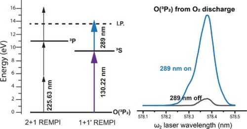
Figure 1. Overview of laser methods used in this study. a) Standard 2 + 1 (left) and threshold 1 + 1' (right) REMPI schemes for O(${}^3{P}_2$) detection. b) Difference frequency four wave mixing scheme for generating 130.22 nm light used in the 1 + 1' scheme. Small changes in the ${\omega }_2$ wavelength (see Figure 2) are used for detection of O(${}^3{P}_{j=0,1}$). c) Energetics of O${}_2$ photodissociation around 130 nm. DL 1, 2, and 3 refer to the (O(${}^{3}P$) + O(${}^{3}P$)), (O(${}^{3}P$) + O(${}^{1}D$)), and (O(${}^{3}P$) + O(${}^{1}S$)) dissociation limits, respectively.

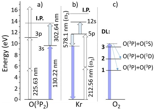
Figure 2. O${}^{+}$ total ion yield spectrum on scanning the ${\omega }_2$ laser wavelength to generate tunable VUV in the vicinity of the $3s{}^3{S}_1^o$ resonance of O(${}^3{P}_j$) atoms.

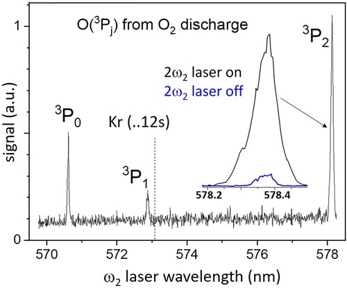
Figure 3. Velocity mapped O${}^{+}$ images (HM geometry), after symmetrisation and correction for the detector inhomogeneity, from O${}_2$ photodissociation with VUV radiation tuned to 1 + 1' REMPI of the O(${}^3{P}_j$) resonances shown in Figure 2. The $\mathbf{E}$ field direction of the linearly polarised VUV radiation is shown on the left and the colour bar on the right codes the signal intensity.

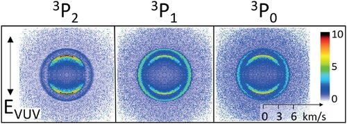
Figure 4. Total kinetic energy release (TKER) distributions from the images shown in Figure 3, after inversion using FINA. The ${}^3{P}_0$ and ${}^3{P}_1$ curves are given a vertical offset for clarity.

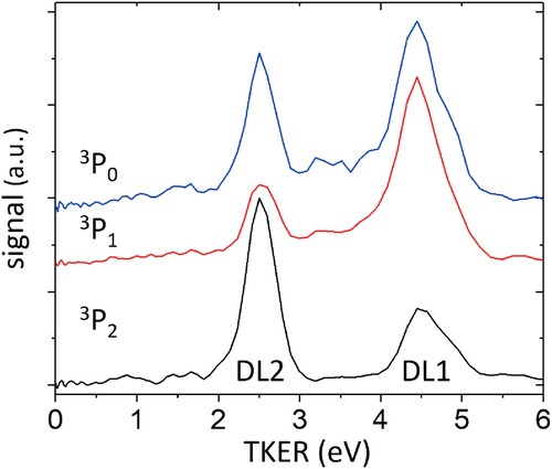
Figure 5. Angular data (scattered points) and fits (solid lines) for the DL 1 and DL 2 recoil rings obtained from the images with HM polarisation shown in Figure 3, after inversion using FINA. Values for ${\text{β}}^{\text{obs}}$ and ${\gamma }^{\text{obs}}$ recovered by the fitting routine are listed in Table 1.

Figure 6. Angular data (scattered points) and fits (solid lines) for the DL 2 recoil ring obtained from the O(${}^3{P}_0$) images with HV (red), HM (blue), and HH (black) polarisation. Values for ${\gamma }^{\text{obs}}$ from the fitting routine are indicated for each curve. The signals for HV and HM polarisation are given a vertical offset for clarity.

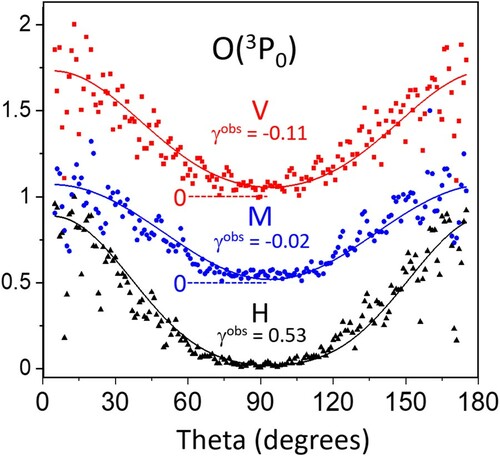
Table 1. Anisotropy parameters β and γ, and fractional populations $A_{\lambda }$ of the different λ levels, where $A_{-\lambda }=A_{\lambda }$, for the different O(${}^3{P}_j$) states for the two different dissociation limits (DL).

State	DL	${\text{β}}^{\text{obs}}$	${\gamma }^{\text{obs}}$	β	$A_0$	$A_1$	$A_2$
${}^3{P}_0$	2	1.8	0.04	1.8	1	–	–
${}^3{P}_0$	1	−0.6	−0.02	−0.6	1	–	–
${}^3{P}_1$	2	1.5	−0.06	1.6	0.4	0.3	–
${}^3{P}_1$	1	−0.3	−0.2	0.5	0.8	0.1	–
${}^3{P}_2$	2	1.8	−0.02	1.8	0.0–0.5	0.3–0.0	0.2–0.3
${}^3{P}_2$	1	0.1	−0.2	0.7	0.0–0.2	0.2–0.0	0.3–0.4
				−0.5	0.4–0.8	0.3–0.0	0.0–0.1

Figure 7. DL 2/total branching ratios in the 127–136 nm region. Closed circles are from the present work with O(${}^3{P}_j$) detection (assuming a statistical j-state distribution), open triangles from [9], open squares from reference [37], and the continuous dashed-line is from reference [38].

H.M. Lambert, A.A. Dixit, E.W. Davis and P.L. Houston, J. Chem. Phys. 121, 10437–10446 (2004).

 PubMed Web of Science ®Google Scholar

L.C. Lee, T.G. Slanger, G. Black and R.L. Sharpless, J. Chem. Phys. 67, 5602–5606 (1977).

 Web of Science ®Google Scholar

J.B. Nee and P.C. Lee, J. Phys. Chem. A 101, 6653–6657 (1997).

 Web of Science ®Google Scholar