Precision measurement of quasi-bound resonances in H₂ and the H + H scattering length

Figures & data

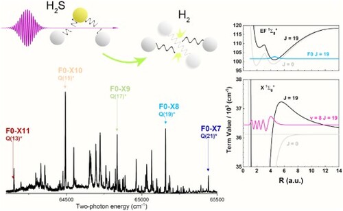
Figure 1. Layout of the experimental setup involving three independently tunable UV-lasers, and a molecular beam apparatus. For details see text.

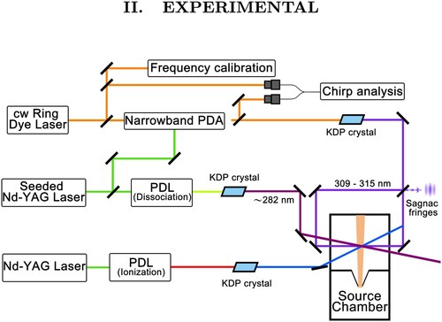
Figure 2. Potential energy surface for the electronic ground states of ${\mathrm{H}}_2$S [47] as a function of the H-H (R) and ${\mathrm{S}-\mathrm{H}}_2$ distance.

Figure 3. Two-photon excitation spectrum of the ${\mathrm{H}}_2$S molecule with probing of ${\mathrm{H}}_2{\mathrm{S}}^{+}$ ion species. The three narrow signals labelled with asterisk corresponding to two-photon transitions in the sulphur atom. See text for details.

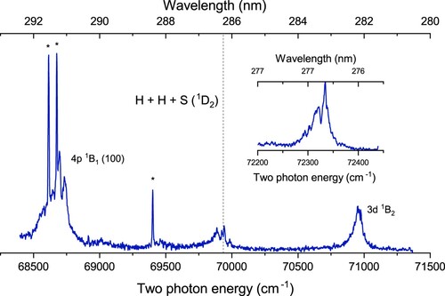
Figure 4. Potential energy curves for the ${\mathrm{X}}^1{\mathrm{\Sigma }}_g^{+}$ ground state and the ${\mathrm{EF}}^1{\mathrm{\Sigma }}_g^{+}$ excited states, drawn for the J = 0 rotationless energies and for higher odd J values, including the centrifugal energy. Also wave functions for a bound X(7,19) and quasi-bound $\mathrm{X}(8,19{)}^{\ast }$ level are displayed. The wave function for the F0(J = 19) excited level (upper panel) indicates overlap at large internuclear separation (4–5 a.u.).

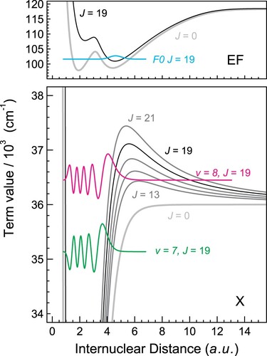
Table 1. Contributions to the dissociation energies of the observed shape resonances of ${\mathrm{H}}_2$ in ${\mathrm{cm}}^{-1}$.

Contribution/$\mathrm{X}(v,J{)}^{\ast }$	(11,13)${}^{\ast }$	(10,15)${}^{\ast }$	(9,17)${}^{\ast }$	(8,19)${}^{\ast }$	(7,21)${}^{\ast }$
$m{\alpha }^2$	−192.2683(29)	−186.1598(36)	−224.5890(40)	−327.0262(43)	−505.4818(45)
Adiabatic	3.1895	4.2857	5.3013	6.2827	7.2555
Nonadiabatic	2.6847	3.2666	3.6583	3.9268	4.1120
$m{\alpha }^4$	−0.2254	−0.2945	−0.3540	−0.4076	−0.4570
BO	−0.2261	−0.2952	−0.3546	−0.4081	−0.4575
Nonadiabatic	0.0007	0.0006	0.0006	0.0005	0.0004
$m{\alpha }^5$	−0.0008	0.0002	0.0021	0.0047	0.0079
$m{\alpha }^6$	−0.0001	−0.0001	−0.0001	−0.0001	−0.0001
Total	−192.4945(29)	−186.4542(36)	−224.9410(40)	−327.4291(43)	−505.9310(45)
Comparison [39]	−192.50	−186.46	−224.95	−327.43	−505.93
${\mathrm{\Gamma }}_{\mathrm{FWHM}}$ (kHz)	$1\times {10}^5$	70	1	0.5	1
Lifetime (s)	$2\times {10}^{-9}$	$2\times {10}^{-6}$	$2\times {10}^{-4}$	$3\times {10}^{-4}$	$2\times {10}^{-4}$

Notes: A negative dissociation energy indicates that these levels lie above the dissociation threshold. A comparison is made with results from Selg [39].

Table 2. Measured frequencies for the two-photon F0-X transitions probing the quasi-bound levels ${\mathrm{H}}_2^{\ast }$, with uncertainties indicated in parentheses. Also some transitions for bound ${\mathrm{H}}_2$ levels are included, relevant for comparison. Computed values from the present work for the F0(J) levels are listed. Term values of the quasi-bound resonances X(v, J)${}^{\ast }$ are obtained from the dissociation energies given in Table 1 and adding the most recent theoretical values for the dissociation energy $D_0=36,118.069605(31){\mathrm{cm}}^{-1}$ [19]. For the bound states values from H2SPECTRE [60,80] are taken. From a combination of these a calculation of two-photon transitions frequencies F0-X can be made. Finally, in the last column the deviations between experimental and predicted frequencies are listed as ${\mathrm{\Delta }}_{\mathrm{Exp}.-\mathrm{Calc}.}$. All values in ${\mathrm{cm}}^{-1}$.

X$(v,J)$	Transition	Exp.	F0(J)${}_{\mathrm{calc}}$	X(v, J)${}_{\mathrm{calc}}^{\ast }$	Calculated	${\mathrm{\Delta }}_{\mathrm{Exp}.-\mathrm{Calc}.}$
(7,21)*	Q(21)	65,441.3575 (9)	102,064.12	36,624.0006	65,440.12	1.24
(7,21)*	O(21)	64,979.430 (10)	101,602.55	36,624.0006	64,978.55	0.88
(8,19)*	Q(19)	65,157.9413 (21)	101,602.55	36,445.4988	65,157.05	0.89
(8,19)*	S(19)	65,619.8599 (8)	102,064.12	36,445.4988	65,618.62	1.24
(8,19)*	O(19)	64,734.8098 (9)${}^a$	101,179.70	36,445.4988	64,734.20	0.61
(9,17)*	Q(17)	64,837.2974 (19)	101,179.70	36,343.0107	64,836.69	0.61
(9,17)*	O(17)	64,454.775 (10)	100,797.40	36,343.0107	64,454.39	0.39
(10,15)*	O(15)	64,152.970 (20)${}^b$	100,457.32	36,304.5238	64,152.80	0.17
(10,15)*	Q(15)	64,493.2404 (9)	100,797.40	36,304.5238	64,492.88	0.36
(11,13)*	Q(13)	64,146.930 (20)${}^b$	100,457.32	36,310.5641	64,146.76	0.17
(8,17)	Q(17)	66,044.7046 (9)	101,179.70	35,135.6038	66,044.10	0.61
(9,15)	Q(15)	65,571.9063 (19)	100,797.40	35,225.8567	65,571.54	0.36
(9,15)	S(15)	65,954.4505 (10)	101,179.70	35,225.8567	65,953.84	0.61

${}^{\mathrm{a}}$Measured both in DC-field free and in DC-field for prompt ion removal.

${}^{\mathrm{b}}$Measured with 3 ns delay, hence temporal overlap, between dissociation laser and spectroscopy laser.

Figure 5. (Left): Overview spectra recorded in a two-laser scheme with two-photon UV-photolysis of ${\mathrm{H}}_2$S, followed by 2+1 REMPI on F-X($v^{\mathrm{\prime }},v^{\mathrm{\prime }\mathrm{\prime }}$) bands with a UV-tunable frequency-doubled dye laser. Transitions are labelled with quantum numbers of the ground level. Excitations from quasi bound resonances are indicated with asterisk (*). The dashed arrows represent the calculated positions of unobserved transitions. (Right): Calculated Franck-Condon factors for the bands F-X(0,$v^{\mathrm{\prime }\mathrm{\prime }}$) as a function of J.

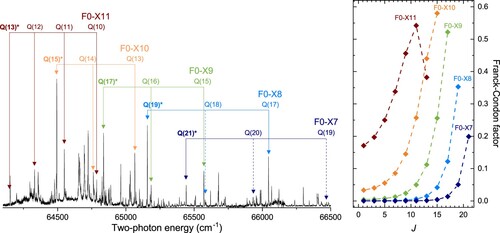
Figure 6. Excitation spectra of two photon transitions in the F-X system probing a number of quasi-bound resonances ${\mathrm{H}}_2^{\ast }$, including from the X(11,13)${}^{\ast }$ short-lived one, and from the bound state X(9,15). The insets show the AC-Stark extrapolation from measurements at varying pulse energies to zero power levels.

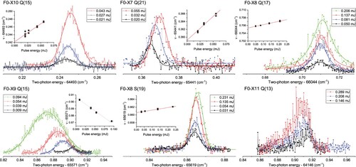
Table 3. Uncertainty budget for the measurements of two-photon F0-X transitions.

Contribution	Uncertainty (MHz)
Lineshape fitting	15
Frequency calibration	9
CW-pulse offset (chirp)	18
Residual Doppler effect	3
DC-Stark effect	<1
Subtotal (exl. AC-Stark)	25
AC-Stark effect	3–60

Note: The uncertainty for the AC-Stark extrapolations is estimated for individual transitions, where the total uncertainties are listed in Table 2.

Figure 7. Two recordings of autoionisation spectra after probing different two-photon transitions in the F-X system, one from the bound X(9,15) state and one from the quasi-bound X(10,15)${}^{\ast }$ resonance. The similarity of the resonances in both spectra and the observation of a Rydberg series converging to the ${\mathrm{X}}^{+}(v^{+}=1,N^{+}=15)$ limit in ${\mathrm{H}}_2^{+}$ proves that a J = 15 state is probed at the intermediate level.

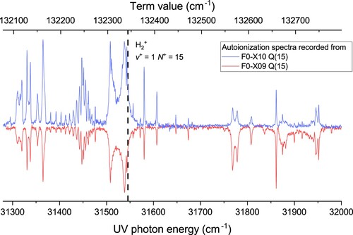
Figure 8. Level diagram of X(v, J) and F0(J) rotational levels with the ${\mathrm{H}}_2$(${\mathrm{X}}^1{\mathrm{\Sigma }}_g^{+}$) dissociation limit given as a dashed line. Measured transitions, plotted as (black) arrows, connect all the observed quasi-bound resonance including measurements of weak S- and O- transitions. The energy splittings are determined from the combination differences and listed in Table 4.

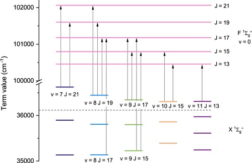
Table 4. Combination differences between ${\mathrm{H}}_2^{\ast }$ quasi-bound resonances, and some bound resonances.

X$(v,J)$	$T_{\mathrm{rel}}^{\exp }$	$T_{\mathrm{rel}}^{\mathrm{calc}}$	$\mathrm{\Delta }T$
(7,21)${}^{\ast }$	319.4772 (28)	319.4768 (9)	0.0004 (29)
(8,17)	−1168.9200 (25)	−1168.9200 (12)	0.0000 (28)
(8,19)${}^{\ast }$	140.9748 (25)	140.9750 (7)	−0.0002 (26)
(9,15)	−1078.6659 (21)	−1078.6671 (11)	0.0012 (24)
(9,17)${}^{\ast }$	38.4872 (30)	38.4869 (4)	0.0003 (30)
(10,15)${}^{\ast }$	0	0	0
(11,13)${}^{\ast }$	6.041 (28)	6.0404 (6)	0.001 (28)

Notes: Level energies are plotted with respect to the $\mathrm{X}(10,15{)}^{\ast }$ resonance. A comparison is made between experimental determination and computed values, while in the last column deviations are given. Note that these discrepancies relate to the inaccuracy in the calculation of F0(J) levels, and not to inaccuracies in the bound and quasi-bound resonances on the ground state potential. All values in ${\mathrm{cm}}^{-1}$.

Figure 9. Upper panel: Range of the BO potential energy curve and the various corrections normalised to $+1$ or $-1$ around the mean internuclear distance for better comparison. Middle panel: R-dependent vibrational and rotational reduced masses, ${\mu }_{\Vert }(R)$ and ${\mu }_{\perp }(R)$, used to take non-adiabatic effects into account within the framework of NAPT. Lower panel: Radial probability density of the v = 0, 3 bound states (black solid line) and the X(11,13) quasi-bound state (coloured solid line). The squared s-wave zero-energy wave function is shown for comparison (dotted line, not to scale).

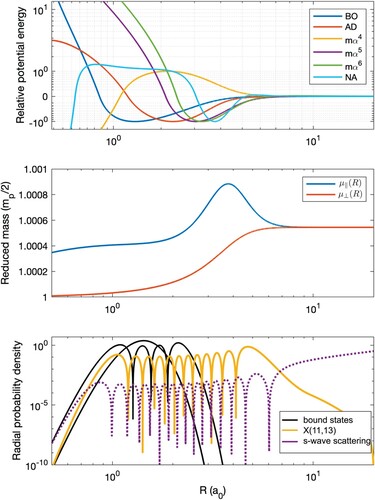
Figure 10. Nonadiabatic, $m{\alpha }^4$, $m{\alpha }^5$ and $m{\alpha }^6$ corrections for the bound states and the long-living quasi-bound states of ${\mathrm{H}}_2$ for J = 0−21. Note that the uncertainties for the separate contributions scale with the actual values plotted here (see text).

G. Tarczay, A.G. Császár, O.L. Polyansky and J. Tennyson, J. Chem. Phys. 115, 1229 (2001). doi:10.1063/1.1379971

 Web of Science ®Google Scholar

M. Selg, J. Chem. Phys, 136, 114113 (2012). doi:10.1063/1.3692968

 Google Scholar

M. Beyer, N. Hölsch, J. Hussels, C.-F. Cheng, E.J. Salumbides, K.S.E. Eikema, W. Ubachs, C. Jungen and F. Merkt, Phys. Rev. Lett. 123, 163002 (2019). doi:10.1103/PhysRevLett.123.163002

 PubMed Web of Science ®Google Scholar

P. Czachorowski, M. Puchalski, J. Komasa and K. Pachucki, Phys. Rev. A 98, 052506 (2018). doi:10.1103/PhysRevA.98.052506

 Web of Science ®Google Scholar

H2SPECTRE ver 7.0 Fortran source code (University of Warsaw, Poland, 2019).

 Google Scholar