Effect of correlated hyperfine theory errors in the determination of rotational and vibrational transition frequencies in HD⁺

Figures & data

Figure 1. Adjustment of $f_{\mathrm{ex},\mathrm{sa}}^{0933}$ and $f_{\mathrm{ex},\mathrm{sa}}^{0001}$ for various correlation scenarios [labelled by the tuples $(r_A,r_B,r_C)$]. The corresponding theoretical predictions $f_{\mathrm{th},\mathrm{sa}}$ are those from Refs. [11,12] and are indicated by the vertical dashed lines, while the shaded area represents the corresponding theoretical uncertainty $u(f_{\mathrm{th},\mathrm{sa}})$. For completeness, a more recent value of $f_{\mathrm{th},\mathrm{sa}}$ by Korobov and Karr [7] is shown as a separate data point. (a) Results for the $(v,N)$: $(0,3)\to (9,3)$ transition, considering correlations only for $E_4^{\rho }$ and $E_5^{\rho }$. The value of $f_{\mathrm{ex},\mathrm{sa}}^{0933}$ as determined by Patra et al. [11] is also indicated. (b) Same as (a), but for the $(v,N)$: $(0,0)\to (0,1)$ transition using the data of Alighanbari et al. [12]. (c) Same as (a), but now considering $E_1^{\rho }$ (type-B correlation only), and the pairs $E_4^{\rho },E_5^{\rho }$ and $E_6^{\rho },E_7^{\rho }$. (d) Same as (b), but now including also type-A correlations between $E_6^{\rho },E_7^{\rho }$.

Figure 2. Results of Monte-Carlo runs. (a) $(v,N)$: $(0,3)\to (9,3)$ transition, 49,701 realisations. (b) $(v,N)$: $(0,0)\to (0,1)$ transition, 49,550 realisations. (c) Zoomed-in portion of the histogram shown in (b).

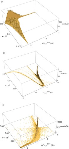
Figure 3. Weight (or probability) w versus r for the Monte-Carlo run shown in Figure 2(a). Although not visible from the graph, the different coloured dots occur in vertically aligned groups of three, each group corresponding to a single adjustment with correlation coefficients $r_A$ (blue), $r_B$ (green), and $r_C$ (red) (colour online only).

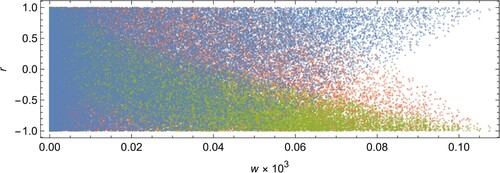
Figure 4. Dependence of the adjusted frequency on the correlation coefficient $r_B$. (a) $\mathrm{\Delta }{\hat{f}}_{\mathrm{ex},\mathrm{sa}}^{0933}$ versus $r_B$ for the scenario $(0,r_B,1)$, and considering correlations between $E_4^{\rho }$ and $E_5^{\rho }$ (upper curve), and between $E_1^{\rho }$, $E_4^{\rho }$, $E_5^{\rho }$, $E_6^{\rho }$, and $E_7^{\rho }$ (lower curve). For the upper and lower curves, the limiting cases $r_B=0$ and $r_B=1$ are also shown in Figure 1(a) and Figure 1(c), respectively. A uniform expansion factor $\eta =1.5$ was applied. (b) $\mathrm{\Delta }{\hat{f}}_{\mathrm{ex},\mathrm{sa}}^{0001}$ versus $r_B$ for the scenario $(1,r_B,1)$, and considering correlations between $E_4^{\rho }$ and $E_5^{\rho }$ (lower curve), and between $E_4^{\rho }$, $E_5^{\rho }$, $E_6^{\rho }$, and $E_7^{\rho }$ (upper curve). In this case, for the lower and upper curves, the limiting cases $r_B=0$ and $r_B=1$ are also shown in Figure 1(b) and Figure 1(d), respectively.

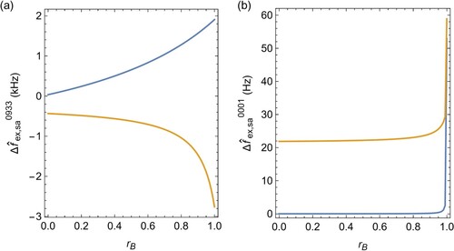
Figure 5. Shift of $\mathrm{\Delta }{\hat{f}}_{\mathrm{ex},\mathrm{sa}}^{0001}$ versus values of $r_A$ (blue), $r_B$ (green), and $r_C$ (red), obtained from Monte-Carlo runs (colour online only). Although not visible from the graphs, the different coloured dots occur in vertically aligned groups of three, each group corresponding to a single adjustment with correlation coefficients $(r_A,r_B,r_C)$. (a) Results of a ∼50,000-point Monte-Carlo run involving $E_4^{\rho }$, $E_5^{\rho }$, $E_6^{\rho }$, and $E_7^{\rho }$. (b) Same as in (a), but now involving only $E_4^{\rho }$ and $E_5^{\rho }$. (c) Same as (a), but now involving only $E_6^{\rho }$ and $E_7^{\rho }$. (d) Weight (or probability) w versus r for the run involving $E_4^{\rho }$, $E_5^{\rho }$, $E_6^{\rho }$, and $E_7^{\rho }$. This run was also used to produce Figure 2(b).

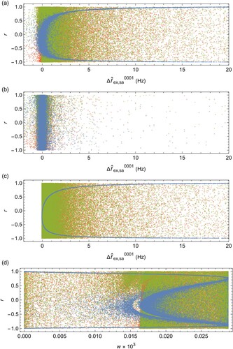
Table 1. Correlation-induced shift and standard uncertainty, as obtained from unweighted and weighted results of the Monte-Carlo runs, to the $(v,N)$: $(0,3)\to (9,3)$ and $(v,N)$: $(0,0)\to (0,1)$ spin-averaged transition frequencies.

	$(v,N)$: $(0,3)\to (9,3)$		$(v,N)$: $(0,0)\to (0,1)$
Method	Shift${}^{\mathrm{a}}$ (kHz)	Uncertainty (kHz)	Shift${}^{\mathrm{b}}$ (Hz)	Uncertainty (Hz)
Monte-Carlo unweighted	−0.07	0.58	1.5	3.6
Monte-Carlo weighted	0.03	0.27	1.1	1.5

${}^{\mathrm{a}}$Shift with respect to ${\hat{f}}_{\mathrm{ex},\mathrm{sa}}^{0933}(0,0,0)=415,264,925,500.7(1.0)$ kHz.

${}^{\mathrm{b}}$Shift with respect to ${\hat{f}}_{\mathrm{ex},\mathrm{sa}}^{0001}(0,0,0)=1,314,925,752,911(17)$ Hz.

Table 2. Correlation-induced shift and standard uncertainty (in ppt), to the value of $m_p/m_e$, as obtained from unweighted and weighted results of the Monte-Carlo runs.

	$(v,N)$: $(0,3)\to (9,3)$		$(v,N)$: $(0,0)\to (0,1)$
Method	Relative shift	Relative uncertainty	Relative shift	Relative uncertainty
Monte-Carlo unweighted	0.5	3.9	$-1.2$	2.8
Monte-Carlo weighted	$-0.2$	1.9	$-0.8$	1.1

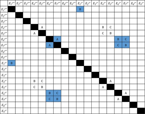
Figure A1. Graphical overview of correlation coefficients. Empty cells correspond to correlation coefficients which are always set to zero, either because the corresponding covariances are negligibly small on an absolute frequency scale, or because the spin coefficients involved are unlikely to be uncorrelated as they represent physically distinct interactions. Nonzero correlations of type A, B and C are indicated. Cells with a shaded background correspond to correlations that are nonzero only in the $(v,N)$: $(0,3)\to (9,3)$ analysis.

S. Patra, M. Germann, J.-Ph. Karr, M. Haidar, L. Hilico, V.I. Korobov, F.M.J. Cozijn, K.S.E. Eikema, W. Ubachs and J.C.J. Koelemeij, Science. 369 (6508), 1238–1241 (2020). doi:10.1126/science.aba0453

 PubMed Web of Science ®Google Scholar

S. Alighanbari, G.S. Giri, F.L. Constantin, V.I. Korobov and S. Schiller, Nature. 581, 152–158 (2020). doi:10.1038/s41586-020-2261-5

 PubMed Web of Science ®Google Scholar

V.I. Korobov and J.-Ph. Karr, Phys. Rev. A. 104, 032806 (2021). doi:10.1103/PhysRevA.104.032806

 Web of Science ®Google Scholar