
Figures & data
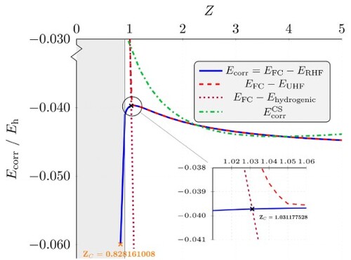
Figure 1. Coordinates utilised in this work (i) Inter-particle coordinates, and
and (ii) Jacobi coordinates
and θ.
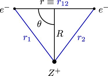
Figure 2. (left) Cartesian coordinate system used in calculating dynamic Coulomb holes. The nucleus is fixed at the origin, electron 1 is fixed on the positive x axis and electron 2 is moved along the x axis. (right) The resulting dynamic Coulomb hole for the helium atom using the Cartesian schematic on the left.
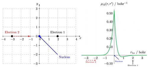
Figure 3. The exact static Coulomb hole curve (solid red line) [Citation23], compared to the difference between the intracule distribution functions and
(solid orange line). The inset plots in (a,b) reveals the secondary Coulomb holes, and the inset plots in (c,d) show a zoom of the primary Coulomb hole region. (a) Li
(b) He (c) H
(d) Z
![Figure 3. The exact static Coulomb hole curve (solid red line) [Citation23], compared to the difference between the intracule distribution functions DFC(r) and DCS(r) (solid orange line). The inset plots in (a,b) reveals the secondary Coulomb holes, and the inset plots in (c,d) show a zoom of the primary Coulomb hole region. (a) Li+ (b) He (c) H− (d) ZCFC](/cms/asset/e3de0531-9904-46b7-a831-bb25a1bbf55e/tmph_a_2146540_f0003_oc.jpg)
Figure 4. The dynamic Coulomb holes for Li (left), He (center), and H
(right); note the different y-axis scales. The nucleus is at the origin, electron 1 is fixed on the positive x axis (indicated by an arrow). Top row corresponds to electron 1 at the most probable distance from the nucleus
, middle row corresponds to the crossing point in the static Coulomb hole
, and row 3 corresponds to electron 1 at 2
.
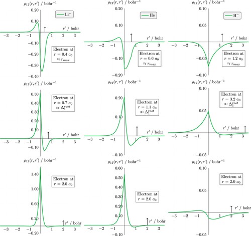
Table 1. Roots, areas and minima of the curves in the helium-like ions in atomic units.
Figure 5. (Left) exact DCH using (Equation13(13)
(13) ) and (right) approximate DCH using (Equation17
(17)
(17) ) for Li
, He and H
. The position of electron 1 is indicated by the circles along the base of each plot. The orange dashed line represents the dynamic Coulomb hole when electron 1 is at
.
![Figure 5. (Left) exact DCH using (Equation13(13) ρ12(r,r′)=ρxc(r,r′)⏟FermiCoulombhole−ρx(r,r′)⏟Fermihole,(13) ) and (right) approximate DCH using (Equation17(17) ρc(r1,r2)=Γ20(r1,r2)[ϕ2(r1,r2)−2ϕ(r1,r2)]ρ0(r1),(17) ) for Li+, He and H−. The position of electron 1 is indicated by the circles along the base of each plot. The orange dashed line represents the dynamic Coulomb hole when electron 1 is at rmax.](/cms/asset/98a5cadd-020c-4f3f-bfea-cd84bac1a7c7/tmph_a_2146540_f0005_oc.jpg)
Figure 6. Electron correlation energies as a function of nuclear charge Z. The black cross corresponds to and the orange cross corresponds to
. The grey shaded region represents unbound systems, i.e. with
[Citation15,Citation37]. The inset provides a zoomed view near the maximum in
.
![Figure 6. Electron correlation energies as a function of nuclear charge Z. The black cross corresponds to ZCHF=1.031177528 and the orange cross corresponds to ZCHF0=0.828161008. The grey shaded region represents unbound systems, i.e. with Z≤0.910 [Citation15,Citation37]. The inset provides a zoomed view near the maximum in Ecorr.](/cms/asset/34be71bc-6550-4061-8780-dc3d51b9082c/tmph_a_2146540_f0006_oc.jpg)
Figure 7. FC and HF radial (intracule) energies, ,
for Li
, He, H
and
. The difference between these two curves (shaded region) represents the electron correlation energy distribution,
, where
. (a) Li
(b) He (c) H
(d) Z
.
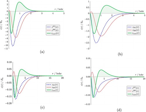
Figure 8. (a) The FC and HF radial (extracule) energies, ,
and electron correlation energy distribution,
, and (b) comparison of
with
calculated using Equation (Equation9
(9)
(9) ). All data are for the helium atom.
![Figure 8. (a) The FC and HF radial (extracule) energies, εFC(R), εHF(R) and electron correlation energy distribution, εcorr(R), and (b) comparison of εcorr(R) with EcorrCS(R) calculated using Equation (Equation9(9) EcorrCS-LYP=−aπ∫γ(R)1+dqρ−1/3(R){ρ(R)+8bq2ρ−5/3(R)[ρα(R)tHFα+ρβ(R)tHFβ−ρ(R)tW(R)]e−cqρ−1/3(R)}dR,(9) ). All data are for the helium atom.](/cms/asset/a34a2bd6-5b30-4082-b397-dec9448add35/tmph_a_2146540_f0008_oc.jpg)
Figure 9. Radial electron correlation energy distributions, , calculated using (a) the CS open-shell energy formula (Equation9
(9)
(9) ) and (b) the LYP functional (Equation10
(10)
(10) ), for anionic (B
, F
), neutral (Li, O) and cationic (C
, N
) atoms. The inset plots show a zoomed view near the origin, highlighting the small positive regions. (a) CS (b) LYP.
![Figure 9. Radial electron correlation energy distributions, Ecorr(R), calculated using (a) the CS open-shell energy formula (Equation9(9) EcorrCS-LYP=−aπ∫γ(R)1+dqρ−1/3(R){ρ(R)+8bq2ρ−5/3(R)[ρα(R)tHFα+ρβ(R)tHFβ−ρ(R)tW(R)]e−cqρ−1/3(R)}dR,(9) ) and (b) the LYP functional (Equation10(10) EcorrLYP=−aπ∫γ(R)1+dqρ−1/3(R){ρ(R)+8bq2ρ−5/3(R)[+118(ρα(R)∇2ρα(R)+ρβ(R)∇2ρβ(R))]e−cqρ−1/3(R)}22/3CFρα8/3(R)+22/3CFρβ8/3(R)−ρ(R)tW+19(ρα(R)tWα(R)+ρβ(R)tWβ(R))+118(ρα(R)∇2ρα(R)+ρβ(R)∇2ρβ(R))]e−cqρ−1/3(R)118}dR,(10) ), for anionic (B−, F−), neutral (Li, O) and cationic (C+, N+) atoms. The inset plots show a zoomed view near the origin, highlighting the small positive regions. (a) CS (b) LYP.](/cms/asset/af5089a8-358c-45b7-993c-79d3d1e4b058/tmph_a_2146540_f0009_oc.jpg)
Table 2. Inter-particle expectation values in atomic units, nucleus-electron cusp (exact value
) and electron-electron cusp
(exact value
), for
, H
, He and Li
using either the fully-correlated (FC), Hartree-Fock (HF) or Colle-Salvetti (CS) wavefunctions.
Data availability statement
The wavefunctions for each system (Li+, He, H- and ZC), along with all the particle density, energy density data, and correlation energy data presented in the paper, are available at http://dx.doi.org/10.25377/sussex.21566013.