Understanding ground and excited-state molecular structure in strong magnetic fields using the maximum overlap method

Figures & data

Figure 1. Schematic of the atom numbering, bond labels and angles in ${\text{H}}_3^{+}$ and H₃.

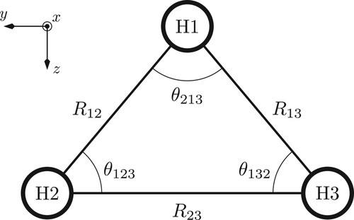
Figure 2. Potential energy curves for equilateral geometries of ${\text{H}}_3^{+}$ calculated using UHF, spin-purified UHF (sp-UHF), and CCSD. (a) The ${}^1{A}_1^{\mathrm{\prime }}$, ${}^1{E}^{\mathrm{\prime }}$ and ${}^3{E}^{\mathrm{\prime }}$ states in the absence of a magnetic field. (b) The corresponding $A^{\mathrm{\prime }}$, ${\mathrm{\Gamma }}^{\mathrm{\prime }}$ and $A^{\mathrm{\prime }}$ states in the presence of a magnetic field of magnitude $0.1B_0$. For states with $M_S=0$, the potential energy curves for the lowest energy orientation with the field vector parallel to the y-axis in Figure 1 is shown. For the state with $M_S=-1$, the lowest energy orientation with the field vector parallel to the x-axis (perpendicular to the molecular plane) is shown. (c) and (d) The corresponding $A^{\mathrm{\prime }}$, ${\mathrm{\Gamma }}^{\mathrm{\prime }}$ and $A^{\mathrm{\prime }}$ states in the presence of a magnetic field of magnitude 0.5 B₀ and 1.0 $B_0$, respectively.

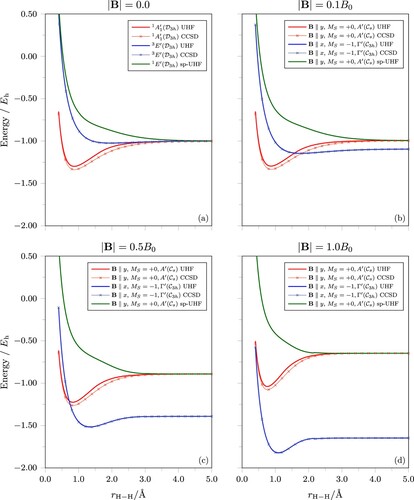
Figure 3. Potential energy curves of the lowest $M_S=-3/2$ state for equilateral geometries of H₃ at various magnetic field strengths. In all finite-field cases, the field vector is parallel to the x-axis and perpendicular to the molecular plane. At zero field, the system has ${\mathcal{D}}_{3h}$ unitary symmetry in which the state is given the symmetry label ${}^4{A}_2^{\mathrm{\prime }}$. At finite fields, the system is reduced to ${\mathcal{C}}_{3h}$ unitary symmetry and the state becomes $A^{\mathrm{\prime }}$ with spin-projection degeneracies lifted. (a) The UHF and CCSD energy curves. (b) The corresponding UHF and CCSD interaction energy curves given by $E(r_{\mathrm{H}-\mathrm{H}})-E(5.0\text{Å})$ plotted on a smaller vertical scale to show the variation of the minimum structures of the UHF and CCSD energy curves in (a) with respect to magnetic field strengths more clearly.

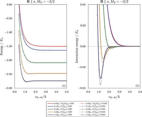
Table 1. Optimised molecular structures for the ${\text{H}}_3^{+}$ and H₃ molecules in particular electronic states as a magnetic field is applied either along the x ($B_x$) or y ($B_y$) directions as shown in Figure 1.

State	$M_S$	$\mathbf{B}/B_0$	Group	Symmetry	Energy / $E_{\mathrm{h}}$	${\theta }_{213}$ / ${}^{\circ }$	${\theta }_{132}$ / ${}^{\circ }$	$R_{12}$ / Å	$R_{23}$ / Å	Shape
${\text{H}}_3^{+}$
${}^1{A}_1^{\mathrm{\prime }}$	0	0	${\mathcal{D}}_{3h}$	$A_1^{\mathrm{\prime }}$	$-1.2985300$ $(-1.3372397)$	60.00	60.00	0.869 (0.878)	0.869 (0.878)	Equilateral
	0	$B_y=0.1$	${\mathcal{C}}_s$	$A^{\mathrm{\prime }}$	$-1.2953725$ $(-1.3340867)$	60.08 (60.09)	59.96 (59.96)	0.867 (0.875)	0.868 (0.877)	Isosceles
	0	$B_y=0.3$	${\mathcal{C}}_s$	$A^{\mathrm{\prime }}$	$-1.2707995$ $(-1.3095510)$	60.67 (60.74)	59.67 (59.63)	0.850 (0.858)	0.858 (0.868)	Isosceles
	0	$B_y=0.5$	${\mathcal{C}}_s$	$A^{\mathrm{\prime }}$	$-1.2246226$ $(-1.2634092)$	61.65 (61.83)	59.18 (59.08)	0.822 (0.830)	0.842 (0.852)	Isosceles
	0	$B_y=0.7$	${\mathcal{C}}_s$	$A^{\mathrm{\prime }}$	$-1.1607536$ $(-1.1995441)$	62.81 (63.13)	58.59 (58.44)	0.790 (0.798)	0.824 (0.835)	Isosceles
	0	$B_y=1.0$	${\mathcal{C}}_s$	$A^{\mathrm{\prime }}$	$-1.0391816$ $(-1.0779118)$	64.64 (65.17)	57.78 (57.42)	0.744 (0.751)	0.796 (0.809)	Isosceles
${}^3{E}^{\mathrm{\prime }}$	$-1$	0	${}^{†}$	–	–	–	–	–	–	–
	$-1$	$B_x=0.1$	${\mathcal{C}}_{3h}$	${\mathrm{\Gamma }}^{\mathrm{\prime }}$	$-1.1453838$ $(-1.1473844)$	60.00	60.00	1.762 (1.739)	1.762 (1.739)	Equilateral
	$-1$	$B_x=0.3$	${\mathcal{C}}_{3h}$	${\mathrm{\Gamma }}^{\mathrm{\prime }}$	$-1.3513473$ $(-1.3546006)$	60.00	60.00	1.516 (1.505)	1.516 (1.505)	Equilateral
	$-1$	$B_x=0.5$	${\mathcal{C}}_{3h}$	${\mathrm{\Gamma }}^{\mathrm{\prime }}$	$-1.5155514$ $(-1.5195295)$	60.00	60.00	1.349 (1.342)	1.349 (1.342)	Equilateral
	$-1$	$B_x=0.7$	${\mathcal{C}}_{3h}$	${\mathrm{\Gamma }}^{\mathrm{\prime }}$	$-1.6517855$ $(-1.6561028)$	60.00	60.00	1.226 (1.222)	1.226 (1.222)	Equilateral
	$-1$	$B_x=1.0$	${\mathcal{C}}_{3h}$	${\mathrm{\Gamma }}^{\mathrm{\prime }}$	$-1.8209581$ $(-1.8254658)$	60.00	60.00	1.093 (1.091)	1.093 (1.091)	Equilateral
${\text{H}}_3$
${}^4{A}_2^{\mathrm{\prime }}$	$-3/2$	0	${}^{†}$	–	–	–	–	–	–	–
	$-3/2$	$B_x=0.5$	${\mathcal{C}}_{3h}$	$A^{\mathrm{\prime }}$	$-2.0882040$ $(-2.0887421)$	60.00	60.00	2.203 (2.144)	2.203 (2.144)	Equilateral
	$-3/2$	$B_x=0.7$	${\mathcal{C}}_{3h}$	$A^{\mathrm{\prime }}$	$-2.2609694$ $(-2.2625532)$	60.00	60.00	1.794 (1.744)	1.794 (1.744)	Equilateral
	$-3/2$	$B_x=1.0$	${\mathcal{C}}_{3h}$	$A^{\mathrm{\prime }}$	$-2.4821822$ $(-2.4857342)$	60.00	60.00	1.445 (1.414)	1.445 (1.414)	Equilateral
	$-3/2$	$B_x=1.1$	${\mathcal{C}}_{3h}$	$A^{\mathrm{\prime }}$	$-2.5472857$ $(-2.5513931)$	60.00	60.00	1.369 (1.342)	1.369 (1.342)	Equilateral
	$-3/2$	$B_x=1.3$	${\mathcal{C}}_{3h}$	$A^{\mathrm{\prime }}$	$-2.6652456$ $(-2.6701932)$	60.00	60.00	1.258 (1.238)	1.258 (1.238)	Equilateral
	$-3/2$	$B_x=1.5$	${\mathcal{C}}_{3h}$	$A^{\mathrm{\prime }}$	$-2.7679688$ $(-2.7735027)$	60.00	60.00	1.179 (1.163)	1.179 (1.163)	Equilateral

${}^{†}$Dissociative.

Notes: Each state is labelled by the spin multiplicity and spatial symmetry that it would adopt in a ${\mathcal{D}}_{3h}$ molecular structure at zero field. Values are computed at the UHF and CCSD levels. CCSD values are shown in parentheses where different.

Figure 4. Variation of the lowest $M_S=-1$ UHF solution of ${\text{H}}_3^{+}$ in the presence of a uniform magnetic field $\mathbf{B}\parallel x$ across a range of ${\theta }_{213}$-constrained geometry-optimised structures. For each constrained value of ${\theta }_{213}$, all three H−H bond lengths in ${\text{H}}_3^{+}$ are allowed to relax to attain an optimal geometry. (a) Energies of the two occupied $m_s=-1/2$ MOs in ${\text{H}}_3^{+}$ along this path, plotted relative to the energy of the HOMO of the ${\theta }_{213}={180}^{\circ }$ geometry-optimised structure in each field strength. The forms of the two β MOs at ${60}^{\circ }$, ${120}^{\circ }$, and ${180}^{\circ }$ are also shown: the isosurface for MO ${\phi }_i(\mathbf{r})$ is plotted at $|{\phi }_i(\mathbf{r})|=0.08$, and the colour at each point $\mathbf{r}$ on the isosurface indicates the phase angle $\arg {\phi }_i(\mathbf{r})\in (-\pi ,\pi ]$ at that point according to the accompanied colour wheel. (b) Energy of the $M_S=-1$ UHF solution along this path, plotted relative to the value at the ${\theta }_{213}={180}^{\circ }$ geometry-optimised structure in each field strength.

Figure 5. Isosurfaces of occupied MOs in the lowest $M_S=-1$ UHF solutions in ${\text{H}}_3^{+}$ and H₂ in the presence of a perpendicular magnetic field. For each molecule, the optimal geometry at $|{\mathbf{B}}_{\perp }|=1.0B_0$ is used to calculate the UHF solution, which is then tracked smoothly to $\mathbf{B}=\mathbf{0}$ with the help of the MOM as the field is switched off while keeping the geometry fixed. This is to generate the corresponding MOs at zero field for investigation purposes. The isosurface for MO ${\phi }_i(\mathbf{r})$ is plotted at $|{\phi }_i(\mathbf{r})|=0.08$, and the colour at each point $\mathbf{r}$ on the isosurface indicates the phase angle $\arg {\phi }_i(\mathbf{r})\in (-\pi ,\pi ]$ at that point according to the colour wheel shown in Figure 4.

${}^{†,‡}$ These MOs turn out to be slightly symmetry-broken at zero field, both of which having actual symmetry $A_1^{\mathrm{\prime }}\oplus E^{\mathrm{\prime }}$. This symmetry breaking, however, is not discernible from the isosurface plots and thus does not affect the qualitative argument given in the main text. Furthermore, as the perpendicular field is introduced, the MOs become symmetry-conserved.

Figure 6. Variation of the lowest $M_S=-3/2$ UHF solution of H₃ in the presence of a uniform magnetic field $\mathbf{B}\parallel x$ across a range of ${\theta }_{213}$-constrained geometry-optimised structures. For each constrained value of ${\theta }_{213}$, all three H−H bond lengths in H₃ are allowed to relax to attain an optimal geometry. (a) Energy of the $M_S=-3/2$ UHF solution along this path, plotted relative to the value at the ${\theta }_{213}={180}^{\circ }$ geometry-optimised structure in each field strength. (b)–(e) Energies of the three occupied β MOs plotted relative to the energy of the HOMO of the ${\theta }_{213}={180}^{\circ }$ geometry-optimised structure in each field strength. The forms of the β MOs at ${60}^{\circ }$, ${120}^{\circ }$, and ${180}^{\circ }$ are also shown: the isosurface for MO ${\phi }_i(\mathbf{r})$ is plotted at $|{\phi }_i(\mathbf{r})|=0.08$, and the colour at each point $\mathbf{r}$ on the isosurface indicates the phase angle $\arg {\phi }_i(\mathbf{r})\in (-\pi ,\pi ]$ at that point according to the colour wheel shown in Figure 4.