Gas-phase electronic spectroscopy of nuclear spin isomer separated H₂O@C₆₀⁺ and D₂O@C₆₀⁺

Figures & data

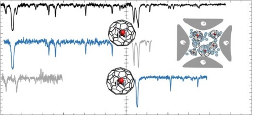
Figure 1. Mass spectrum recorded after storage of H${}_2$O@C${}_{60}^{+}$ in helium buffer gas at 4 K.

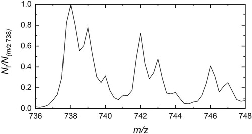
Figure 2. The electronic spectrum of C${}_{60}^{+}$ (top) and H${}_2$O@C${}_{60}^{+}$ (bottom), recorded under the same laboratory conditions. The data are photofragmentation spectra of C${}_{60}^{+}$−He and H${}_2$O@C${}_{60}^{+}$−He complexes.

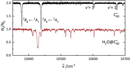
Table 1. Vibrational and translational modes obtained from calculations.

	B3LYP/6-31++G**
Mode	H${}_2$O@C${}_{60}^{+}$	D${}_2$O@C${}_{60}^{+}$
T${}_1$/cm${}^{-1}$	125	115
T${}_2$/cm${}^{-1}$	126	120
T${}_3$/cm${}^{-1}$	128	119
${\nu }_1$/cm${}^{-1}$	111	80
${\nu }_2$/cm${}^{-1}$	101	73
${\nu }_3$/cm${}^{-1}$	34	26

Figure 3. Number of H${}_2$O@C${}_{60}^{+}$−He complexes (N${}_i$) as a function of laser fluence upon irradiation at 10,438 cm${}^{-1}$. Without exposure to laser radiation, 1100±60 ions with m/z = 742 were in the trap. 800±30 complexes remain after irradiation, corresponding to 73±5% of the population.

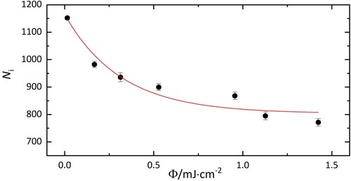
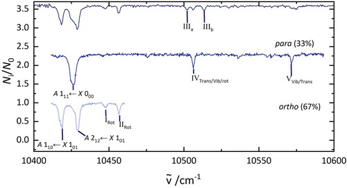
Figure 4. Electronic spectra of H${}_2$O@C${}_{60}^{+}$ (top), p-H${}_2$O@C${}_{60}^{+}$ (middle), and o-H${}_2$O@C${}_{60}^{+}$ (bottom). The lower two traces were obtained in 2 colour experiments. The middle spectrum was recorded by fragmenting all complexes that absorb at 10,429 cm${}^{-1}$. The bottom spectrum was recorded after irradiation at 10,438 cm${}^{-1}$.

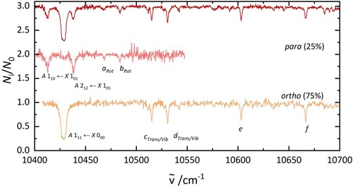
Figure 5. PGopher simulations of the rotational pattern of an electronic transition of H${}_2$O. The details of the simulations are explained in the text. The middle trace uses the parameters based on a geometry optimisation (B3LYP/6-31++G**) while the upper one shows a fit involving a geometry change of H${}_2$O between ground and excited state.

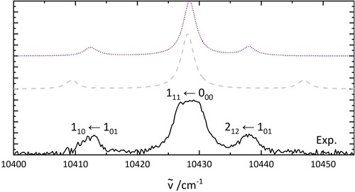
Table 2. Rotational constants used for the simulation in Figure 5.

Constant	H${}_2$O@C${}_{60}^{+}$ /cm${}^{-1}$	D${}_2$O@C${}_{60}^{+}$/cm${}^{-1}$
ΔE	10,394.83*	10,412.15*
A${}_X$	27.25	13.63
B${}_X$	14.25	7.13
C${}_X$	9.36	4.68
A${}_A$	27.25	11*
B${}_A$	13.98*	5.38*
C${}_A$	6.35*	2.75*

Notes: Values without * are taken from the optimised geometry. * indicates free parameters that were obtained during the fit. Subscript ${}_X$ and ${}_A$ refer to the ground and excited state, respectively.

Table 3. Absorption energies and proposed assignment of bands in the H${}_2$O@C${}_{60}^{+}$ and D${}_2$O@C${}_{60}^{+}$ spectra.

H${}_2$O@C${}_{60}^{+}$	$\tilde{\nu }$/cm${}^{-1}$	D${}_2$O@C${}_{60}^{+}$	$\tilde{\nu }$/cm${}^{-1}$	Assignments
	10,412		10,418	Rot	($A{1}_{10}\leftarrow X{1}_{01}$)
	10,429		10,426	Rot	($A{1}_{11}\leftarrow X{0}_{00}$)
	10,438		10,429	Rot	($A{2}_{12}\leftarrow X{1}_{01}$)
a	10,469	I	10,447	Rot	($A{2}_{21}\leftarrow X{1}_{10}$)
					($A{2}_{11}\leftarrow X{1}_{01}$)
b	10,484	II	10,457	Rot	($A{2}_{21}\leftarrow X{1}_{10}$)
					($A{2}_{21}\leftarrow X{1}_{01}$)
					($A{3}_{03}\leftarrow X{1}_{01}$)
					($A{2}_{20}\leftarrow X{1}_{01}$)
c	10,516	III${}_a$	10,502	Tr/Vib
d	10,531	III${}_b$	10,513	Tr/Vib
		IV	10,506	Vib
e	10,603	V	10,571	Vib
f	10,666		–	Cage

Notes: There are several possible assignments for bands a-f . See the text for a discussion.

Figure 6. A comparison of the electronic spectrum of H${}_2$O@C${}_{60}^{+}$ (top) and D${}_2$O@C${}_{60}^{+}$ (bottom) recorded under similar laboratory conditions. The labels are discussed in the text.

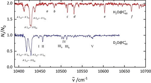
Figure 7. PGopher simulations of the rotational pattern of an electronic transition of D${}_2$O in comparison with the experimental results on D${}_2$O@C${}_{60}^{+}$ (bottom). The rotational constants for the simulation are derived as described in the text.

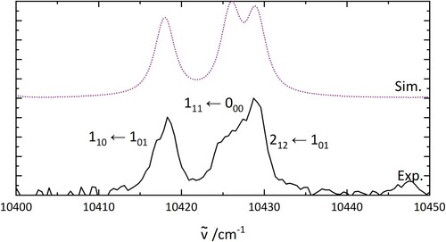
Figure 8. Electronic spectra of D${}_2$O@C${}_{60}^{+}$ (top), para-D${}_2$O@C${}_{60}^{+}$ (middle), and ortho-D${}_2$O@C${}_{60}^{+}$(bottom). The middle trace was recorded by fragmenting all complexes that absorb at 10,418 cm${}^{-1}$ and the bottom trace was recorded by irradiating at 10,426 cm${}^{-1}$.