Modelling of adsorbate-size dependent explicit isotherms using a segregated approach to account for surface heterogeneities

Figures & data

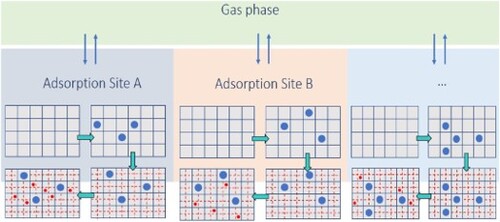
Figure 1. Equilibrium of each of the adsorbed phases with the gas phase in the Segregated Ideal Adsorbed Solution Theory (SIAST) model [22]. Each adsorbed phase is separately in equilibrium with the gas phase. The system is at a constant temperature. The gas phase has a total pressure of $p_{\mathrm{tot}}$ and the mole fraction of component i equals $y_i$. In the adsorbed phase j, the loading of component i is $q_{i,j}$.

Figure 2. Representation of the adsorbent as a lattice where species of different sizes are adsorbed [34]. (a) The adsorbent is divided into $M_1$ sites. (b) adsorption of N indistinguishable molecules of species 1, represented by the blue circles, is taking place on the lattice. (c) After the adsorption of N molecules of species 1, the remaining lattice sites are further divided into $(n{M}_1-nN)$ sites. (d) adsorption of K indistinguishable molecules of species 2 is taking place on the lattice. The blue circles represent species 1 and the smaller red circles represent species 2.

Figure 3. Representation of Segregated Explicit Isotherm (SEI) model which accounts for the separate thermodynamic equilibria of the adsorbed phases with the gas phase at different adsorption sites. Each adsorbed phase is separately in thermodynamic equilibrium with the gas phase and it is represented by the adsorption isotherm proposed by Van Assche et al. [34] Equation (23(23) $q_i=\left(q_{\max ,1}{k}_i{p}_i\right)\frac{\left[\prod _{m=1}^i{\alpha }_m\right]}{\beta }$(23) ). The gas phase has a total pressure of $p_{\mathrm{tot}}$ and the gas phase mole fractions of the components in the mixture are represented by $y_i$. In the adsorbed phase j, the loading of the component i is $q_{i,j}$.

Table 1. Input parameters for the simulation of the breakthrough curve (catalyst particle density, $({\rho }_{\mathrm{p}})$, bed voidage $({\epsilon }_{\mathrm{b}})$, interstitial velocity at the inlet, $(v_{\mathrm{in}})$, and total pressure $(p_{\mathrm{tot}})$) for both cases.

	${\rho }_{\mathrm{p}}[\mathrm{kg}/{\mathrm{m}}^3]$	${\epsilon }_{\mathrm{b}}$	$v_{\mathrm{in}}[\mathrm{m}/\mathrm{s}]$	$p_{\mathrm{tot}}[\mathrm{bar}]$
${\mathrm{CO}}_2-{\mathrm{C}}_3$	1711.06	0.128	0.1	1.0
${\mathrm{nC}}_4-{2\mathrm{mC}}_3$	1796.34	0.40	0.1	10.0

Table 2. Mass transfer coefficients $(k_{\mathrm{M}})$ for the components in both the case studies.

	${\mathrm{CO}}_2$	${\mathrm{C}}_3$	${\mathrm{nC}}_4$	${2\mathrm{mC}}_3$
$k_{\mathrm{m}}[1/\mathrm{s}]$	0.06	0.06	0.06	0.06

Figure 4. Pure component adsorption isotherms of ${\mathrm{CO}}_2$ and ${\mathrm{C}}_3$ in MOR-type zeolite at 300K. Pure component adsorbed loadings calculated using GCMC for the pressure range $({10}^0-5\cdot {10}^{10})$ Pa are fitted to the dual-site Langmuir isotherms. The empty circles represent GCMC simulation data and the solid lines are the dual-site Langmuir isotherms fitted to these data sets. The results obtained in this work are in excellent agreement with the data published by Swisher et al. [22].

Table 3. Fitted parameters for the adsorption of pure ${\mathrm{CO}}_2$ and ${\mathrm{C}}_3$ in MOR-type zeolite at 300 K.

	$k_1[1/\mathrm{Pa}]$	$q_{\max ,1}[\mathrm{mol}/(\mathrm{kgframework})]$	$k_2[1/\mathrm{Pa}]$	$q_{\max ,2}[\mathrm{mol}/(\mathrm{kgframework})]$
${\mathrm{CO}}_2$	$2.617\cdot {10}^{-4}$	1.60	$4.859\cdot {10}^{-7}$	3.62
${\mathrm{C}}_3$	$6.506\cdot {10}^{-9}$	1.73	$2.376\cdot {10}^{-4}$	1.09

Notes: Adsorbed loadings obtained from the GCMC simulations for the pressure range $({10}^0-5\cdot {10}^{10})$ Pa are fitted using the dual-site Langmuir isotherm. Subscript 1 indicates site 1 (smaller pockets) and subscript 2 indicates site 2 (larger pockets) present inside MOR-type zeolite. (See also Figure 5.).

Figure 5. Snapshots of adsorption of pure CO${}_2$ and C${}_3$ molecules in MOR-type zeolite at 300K using GCMC simulations. (a) adsorption of ${\mathrm{CO}}_2$ at ${10}^3$Pa, (b) adsorption of ${\mathrm{CO}}_2$ at ${10}^9$Pa, (c) adsorption of ${\mathrm{C}}_3$ at ${10}^3$Pa and (d) adsorption of ${\mathrm{C}}_3$ at ${10}^9$Pa. Site 1 represents the smaller pockets and site 2 represents the larger pockets inside MOR-type zeolite

Figure 6. Adsorption isotherms of an equimolar mixture ${\mathrm{CO}}_2$ and ${\mathrm{C}}_3$ (50:50) in MOR-type zeolite at 300K. A comparison is made between the adsorbed loadings calculated using GCMC, IAST, SIAST and SEI. The pressure range $({10}^2-{10}^8)$ Pa is considered for the calculations performed using IAST, SIAST and SEI. For GCMC simulations, the pressure range is $({10}^4-{10}^8)$ Pa. Cross marks represent GCMC calculations, triangles are used for IAST, circles for SIAST and squares for SEI.

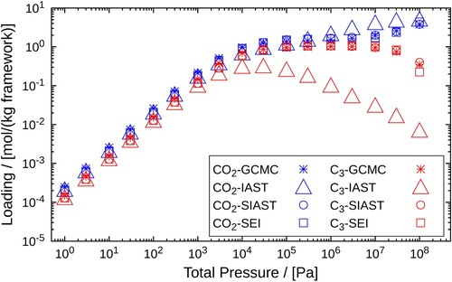
Figure 7. Pure component adsorption isotherms of ${\mathrm{nC}}_4$ and ${2\mathrm{mC}}_3$ in MFI-type zeolite at 400K. Pure component adsorbed loadings calculated using GCMC for the pressure range $({10}^0-5\cdot {10}^{10})$ Pa are fitted using the dual-site Langmuir isotherms. The empty circles represent GCMC simulation data and the solid lines are the dual-site Langmuir isotherms fitted to these data sets.

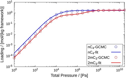
Table 4. Fitted parameters for the adsorption of pure ${\mathrm{C}}_4$ and $2\mathrm{m}{\mathrm{C}}_3$ in MFI-type zeolite at 400K.

	$k_1[1/\mathrm{Pa}]$	$q_{\max ,1}[\mathrm{mol}/(\mathrm{kgframework})]$	$k_2[1/\mathrm{Pa}]$	$q_{\max ,2}[\mathrm{mol}/(\mathrm{kgframework})]$
${\mathrm{nC}}_4$	$2.552\cdot {10}^{-4}$	0.70	$2.348\cdot {10}^{-5}$	1.02
${2\mathrm{mC}}_3$	$9.861\cdot {10}^{-5}$	0.70	$1.00\cdot {10}^{-7}$	0.90

Notes: Adsorbed loadings obtained from the GCMC simulations for the pressure range of $({10}^0-5\cdot {10}^{10})$ Pa are fitted using the dual-site Langmuir isotherm. Subscript 1 indicates site 1 (intersections between the channels) and subscript 2 indicates site 2 (channels) present inside MFI-type zeolite.

Figure 8. Typical snapshots of adsorption of pure C${}_4$ and 2mC${}_3$ molecules in MFI-type zeolite at 400K using GCMC simulations. (a) adsorption of ${\mathrm{C}}_4$ at ${10}^4$Pa, (b) adsorption of ${\mathrm{C}}_4$ at ${10}^8$Pa, (c) adsorption of ${2\mathrm{mC}}_3$ at ${10}^4$Pa and (d) adsorption of ${2\mathrm{mC}}_3$ at ${10}^8$Pa. Site 1 represents the intersections and site 2 represent the channels present inside the MFI-type zeolite.

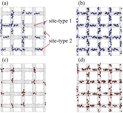
Figure 9. Adsorption isotherms of an equimolar mixture ${\mathrm{nC}}_4$ and ${2\mathrm{mC}}_3$ in MFI-type zeolite at 400K. A comparison is drawn between the adsorbed loadings calculated using GCMC, IAST, SIAST and SEI. The pressure range $({10}^2-{10}^8)$ Pa is considered for the calculations performed using IAST, SIAST and SEI. For GCMC simulations, the pressure range is $({10}^4-{10}^8)$ Pa. Cross marks represent GCMC calculations, triangles are used for IAST, circles for SIAST and squares for SEI.

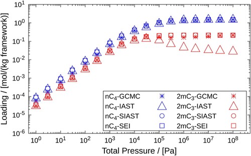
Figure 10. Comparison of breakthrough curves obtained on implementing IAST, SIAST and SEI to the breakthrough curve model. Separation of (a) ${\mathrm{CO}}_2$-${\mathrm{C}}_3$ mixture using MOR-type zeolite at 300K and ${10}^5$Pa, (b) ${\mathrm{nC}}_4$-${2\mathrm{mC}}_3$ mixture using MFI-type zeolite at 400K and ${10}^6$Pa. Each component constitutes $10\mathrm{\%}$ of the mixture in the gas phase. The remaining amount is a non adsorbing carrier gas (helium). Solid lines represent the implementation of SEI. Dashed-dotted lines are used for the SIAST model and dashed lines are used for the IAST model.

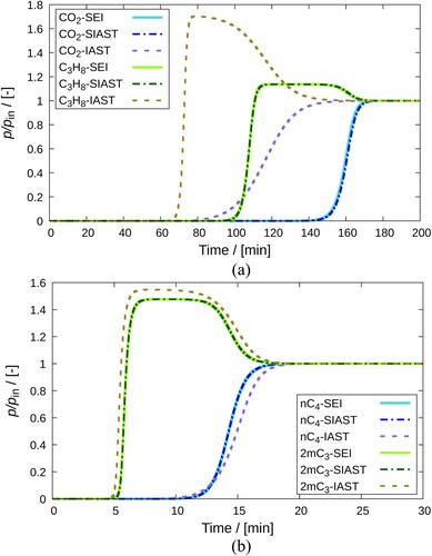
Table 5. Variation in simulation run time $(t_{\mathrm{run}})$ for the breakthrough curve model on implementing SEI, SIAST and IAST.

	$t_{\mathrm{run}}[\mathrm{hrs}](\mathrm{case}1)$	$t_{\mathrm{run}}[\mathrm{hrs}](\mathrm{case}2)$
$\mathrm{IAST}$	17.4	2.94
$\mathrm{SIAST}$	0.92	0.15
$\mathrm{SEI}$	0.33	0.05

Notes: Comparisons are drawn for both case studies: ${\mathrm{CO}}_2-{\mathrm{C}}_3$ (case 1) and ${\mathrm{nC}}_4-{2\mathrm{mC}}_3$ mixtures (case 2). These simulations were run on a local supercomputer at Delft University of Technology (HAL9000).

J.A. Swisher, L.C. Lin, J. Kim and B. Smit, AICHE J 59, 3054–3064 (2013). doi:10.1002/aic.14058.

 Web of Science ®Google Scholar

T.R.C. Van Assche, G.V. Baron and J.F.M. Denayer, Adsorption 24, 517–530 (2018). doi:10.1007/s10450-018-9962-1.

 Web of Science ®Google Scholar