Influence of Regge poles on rainbow angular scattering for state-to-state chemical reactions using Heisenberg’s S matrix programme

Figures & data

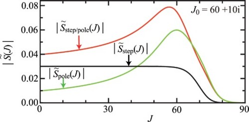
Figure 1. S matrix data for the smooth-step parameterisation. The values of the parameters are given in section 7. (a) $|{\tilde{S}}_{\text{step}}\left(J\right)|$ versus $J$. (b) $\arg {\tilde{S}}_{\text{step}}\left(J\right)/\text{rad}$ versus $J$. The maximum and local minimum of the $\arg {\tilde{S}}_{\text{step}}\left(J\right)/\text{rad}$ curve define the glory angular momentum variables, $J_{{\text{g}}_1}$ and $J_{{\text{g}}_2}$, respectively, which are indicated by orange dashed lines and arrows. The rainbow angular momentum variable, $J_{\text{r}}$, is indicated by a pink dashed line and arrow. (c) ${\tilde{\mathrm{\Theta }}}_{\text{step}}\left(J\right)/\mathrm{deg}$ versus $J$. The red dashed line and arrow indicate $+{\theta }_{\text{R}}$ and $J_1=J_1\left({\theta }_{\text{R}}\right)$ for the N scattering. The blue dashed line and arrows indicate $-{\theta }_{\text{R}}$ as well as $J_2=J_2\left({\theta }_{\text{R}}\right)$ and $J_3=J_3\left({\theta }_{\text{R}}\right)$ for the F scattering. Also shown is $J_{\text{r}}$, which is located at the minimum of the ${\tilde{\mathrm{\Theta }}}_{\text{step}}\left(J\right)/\mathrm{deg}$ curve, where ${\tilde{\mathrm{\Theta }}}_{\text{step}}\left(J=J_{\text{r}}\right)=-{\theta }_{\text{R}}^{\text{r}}$(pink arrow and dashed lines) together with $J_{{\text{g}}_1}$ and $J_{{\text{g}}_2}$, which satisfy ${\tilde{\mathrm{\Theta }}}_{\text{step}}\left(J_{{\text{g}}_1}\text{or}{J}_{{\text{g}}_2}\right)=0$. The three branches of the deflection function are labelled 1 (N, red) and 2, 3 (F, both blue). (d) $\left(2J+1\right)|{\tilde{S}}_{\text{step}}\left(J\right)|$ versus $J$. Also marked are, $J_{{\text{g}}_1}$, $J_{\text{r}}$, $J_{{\text{g}}_2}$, with dashed lines and arrows, and the N and F angular zones. [See colour online].

Figure 2. Plots of PWS dDCSs and PWS LAMs versus ${\theta }_{\text{R}}$, for the smooth-step parameterisation. The values of the parameters are given in section 7. (a) Logarithmic plots of the full and N,F dDCSs for the angular range, ${\theta }_{\text{R}}=0^{\circ }-{180}^{\circ }$, for resummation parameters of $r=0$,1,2,3, together with the rainbow angle, ${\theta }_{\text{R}}^{\text{r}}={40.0}^{\circ }$. (b) Logarithmic plots of the full and N,F dDCSs for the angular range, ${\theta }_{\text{R}}=0^{\circ }-{60}^{\circ }$, for $r=1$. (c) Plots of the full and N,F LAMs for the angular range, ${\theta }_{\text{R}}=0^{\circ }-{180}^{\circ }$, with r = 1. The light blue curve indicates the angular range where the F LAM is non-physical. (d) Plots of the full and N,F LAMs for the angular range, ${\theta }_{\text{R}}=0^{\circ }-{60}^{\circ }$, with $r=1$. The pink arrows at ${\theta }_{\text{R}}\approx {35.6}^{\circ }$ and ${\theta }_{\text{R}}\approx {20.8}^{\circ }$ in (b) and (d) indicate the positions of the maxima for the primary rainbow and first supernumerary rainbow, respectively, for the uAiry asymptotic (SC) approximation of Section 6.3. [See colour online].

Figure 3. Comparison of PWS and SC results for dDCSs and LAMs, all plotted versus ${\theta }_{\text{R}}$, for the smooth-step parameterisation. The values of the parameters are given in Section 7. (a) Full PWS dDCS and full, N,F SC dDCSs for the angular range, ${\theta }_{\text{R}}=0^{\circ }-{180}^{\circ }$. (b) Full PWS and full, N,F SC dDCSs for the angular range, ${\theta }_{\text{R}}=0^{\circ }-{60}^{\circ }$. (c) Full PWS LAM and full, N,F SC LAMs for the angular range, ${\theta }_{\text{R}}=0^{\circ }-{180}^{\circ }$. (d) Full PWS LAM and full, N,F SC LAMs for the angular range, ${\theta }_{\text{R}}=0^{\circ }-{60}^{\circ }$. The pink arrows at ${\theta }_{\text{R}}\approx {35.6}^{\circ }$ and ${\theta }_{\text{R}}\approx {20.8}^{\circ }$ in (b) and (d) indicate the positions of the maxima for the primary rainbow and first supernumerary rainbow, respectively, for the uAiry asymptotic (SC) approximation of Section 6.3. The pink arrows mark the rainbow angle, ${\theta }_{\text{R}}^{\text{r}}={40.0}^{\circ }$. [See colour online].

Figure 4. S matrix data for the pole parameterisation, with $J_0=60+10\text{i}$ and ${\tilde{a}}_0=1$. (a) Argand diagram for ${\tilde{s}}_{\text{pole}}\left(J\right)$. (b) $\arg {\tilde{s}}_{\text{pole}}\left(J\right)/\text{rad}$ versus $J$. (c) $|{\tilde{s}}_{\text{pole}}\left(J\right)|$ versus $J$. (d) ${\tilde{\mathrm{\Theta }}}_{\text{pole}}\left(J\right)/\mathrm{deg}$ versus J, with 2 and 3 indicating the two branches on the F of the deflection function. Also shown as a pink dashed line and arrow are the rainbow angular momentum variable and negative rainbow angle, $J_{\text{r}}\left(\text{pole}\right)$ and $-{\theta }_{\text{R}}^{\text{r}}\left(\text{pole}\right)=-{5.7}^{\circ }$, respectively. In (a), (b), (c), the black solid circles are for $J=0\left(1\right)120$, with the black arrow showing the direction of increasing $J$. The black solid lines are the corresponding loci. [See colour online].

Figure 5. S matrix data for the pole parameterisation, with $J_0=60+10\text{i}$ and ${\tilde{a}}_0=6.428+7.660\text{i}$. (a) Argand diagram for ${\tilde{s}}_{\text{pole}}\left(J\right)$. (b) $\arg {\tilde{s}}_{\text{pole}}\left(J\right)/\text{rad}$ versus $J$. (c) $|{\tilde{s}}_{\text{pole}}\left(J\right)|$ versus $J$. (d) ${\tilde{\mathrm{\Theta }}}_{\text{pole}}\left(J\right)/\mathrm{deg}$ versus $J$, with 2 and 3 indicating the two branches on the F of the deflection function. Also shown as a pink dashed line and arrow are the rainbow angular momentum variable and negative rainbow angle, $J_{\text{r}}\left(\text{pole}\right)$ and $-{\theta }_{\text{R}}^{\text{r}}\left(\text{pole}\right)=-{5.7}^{\circ }$, respectively. In (a), (b), (c), the black solid circles are for $J=0\left(1\right)120$, with the black arrow showing the direction of increasing $J$. The black solid lines are the corresponding loci. [See colour online].

Figure 6. ${\tilde{\mathrm{\Theta }}}_{\text{pole}}\left(J\right)/\mathrm{deg}$ versus $J$ for $J_0=60+2\text{i}$ and ${\tilde{a}}_0=1$ plotted as a blue solid curve. Labels 2 and 3 indicate the two branches for the F of the deflection function. Also shown as a pink dashed line and pink arrow are the rainbow angular momentum variable and negative rainbow angle, $J_{\text{r}}\left(\text{pole}\right)$ and $-{\theta }_{\text{R}}^{\text{r}}\left(\text{pole}\right)=-{28.6}^{\circ }$, respectively. The vertical green solid lines are drawn from the $J$ axis to approximately the full width at half depth of the ‘valley’, and show that 5 partial waves contribute, namely, $J=58$, 59, 60, 61, 62. [See colour online].

Figure 7. S matrix data for the pole, step and step/pole ≡ s/p parameterisations. The pole parameterisation has, $J_0=60+10\text{i}$, and ${\tilde{a}}_0=-18.794-6.840\text{i}$. (a) Plots of $|{\tilde{S}}_{\text{pole}}\left(J\right)|$, $|{\tilde{S}}_{\text{step}}\left(J\right)|$, $|{\tilde{S}}_{\text{step/pole}}\left(J\right)|$, versus $J$. (b) $\tilde{\mathrm{\Theta }}\left(J\right)/\mathrm{deg}$ versus $J$ for the step (black dashed curve) and step/pole (red solid curve for N and blue solid curve for F) parameterisations. Also marked are, $J_{{\text{g}}_1}$, $J_{\text{r}}$, $J_{{\text{g}}_2}$, $-{\theta }_{\text{R}}^{\text{r}}=-{44.5}^{\circ }$, by arrows and a dashed line. The three branches of the defection functions are labelled 1 (N, red) and 2, 3 (F, both blue). (c) $\left(2J+1\right)|{\tilde{S}}_{\text{step/pole}}\left(J\right)|$ versus $J$. [See colour online].

Figure 8. Logarithmic PWS and SC results for dDCSs, all plotted versus ${\theta }_{\text{R}}$, for the step/pole parameterisation. The pole parameterisation has, $J_0=60+10\text{i}$, and ${\tilde{a}}_0=-18.794-6.840\text{i}$. The pink arrows show the rainbow angle at ${\theta }_{\text{R}}^{\text{r}}={44.5}^{\circ }$. (a) Full PWS dDCS for the step/pole parameterisation (black solid curve). Also shown is the full PWS dDCS for the step parameterisation (black dashed curve) in both cases for the angular range, ${\theta }_{\text{R}}=0^{\circ }-{90}^{\circ }$. (b) Full PWS dDCS (black) and PWS N(red), F(blue) $r=1$ dDCSs for the angular range, ${\theta }_{\text{R}}=0^{\circ }-{180}^{\circ }$. (c) Full PWS dDCS (black) and full SC dDCS (green) for the angular range, ${\theta }_{\text{R}}=0^{\circ }-{90}^{\circ }$. (d) Full PWS and PWS N (red solid curve), F(blue solid curve) $r=1$ dDCSs compared with SC N(red dashed curve, denoted SC/N/PSA), F (cyan solid curve for uAiry, and blue dashed curve for tAiry) dDCSs for the angular range, ${\theta }_{\text{R}}=0^{\circ }-{90}^{\circ }$. [See colour online].

Figure 9. S matrix data for the pole, step and step/pole ≡ s/p parameterisations. The pole parameterisation has, $J_0=60+2\text{i}$, and ${\tilde{a}}_0=1.277-4.834\text{i}$. (a) Plots of $|{\tilde{S}}_{\text{pole}}\left(J\right)|$, $|{\tilde{S}}_{\text{step}}\left(J\right)|$, $|{\tilde{S}}_{\text{step/pole}}\left(J\right)|$, versus $J$. (b) $\tilde{\mathrm{\Theta }}\left(J\right)/\mathrm{deg}$ versus $J$ for the step (black dashed curve) and step/pole (red solid curve for N and blue solid curve for F) parameterisations. Also marked are, $J_{{\text{g}}_1}$, $J_{\text{r}}$, $J_{{\text{g}}_2}$, $-{\theta }_{\text{R}}^{\text{r}}=-{60.7}^{\circ }$, by arrows and a dashed line. The three branches of the deflection functions are labelled 1 (N, red) and 2, 3 (F, both blue). (c) $\left(2J+1\right)|{\tilde{S}}_{\text{step/pole}}\left(J\right)|$ versus $J$. [See colour online].

Figure 10. Logarithmic PWS and SC results for dDCSs, for the step/pole parameterisation, all plotted versus ${\theta }_{\text{R}}$ for the angular range, ${\theta }_{\text{R}}=0^{\circ }-{180}^{\circ }$. The pole parameterisation has, $J_0=60+2\text{i}$, and ${\tilde{a}}_0=1.277-4.834\text{i}$. The pink arrows show the rainbow angle at ${\theta }_{\text{R}}^{\text{r}}={60.7}^{\circ }$. (a) Full PWS dDCS for the step/pole parameterisation (black solid curve). Also shown is the full PWS dDCS for the step parameterisation (black dashed curve). (b) Full PWS dDCS (black) and PWS N (red), F (blue) $r=1$ dDCSs. (c) Full PWS dDCS (black) and full SC dDCS (green). (d) Full PWS and PWS N (red solid curve), F (blue solid curve) $r=1$ dDCSs compared with SC N (red dashed curve, denoted SC/N/PSA), F (cyan solid curve for uAiry, and blue dashed curve for tAiry) dDCSs. [See colour online].

Table 1. Numerical values of the Regge pole positions and partial residues for n = 0, 1, 2, 3, 4, 5.

n	$J_n$	$\mathrm{R}\mathrm{e}{\tilde{a}}_n$	$\mathrm{Im}{\tilde{a}}_n$
0	60 + 10i	−2272.83	4453.56
1	60 + 12i	11364.2	−22267.8
2	60 + 14i	−22728.3	44535.6
3	60 + 16i	22728.3	−44535.6
4	60 + 18i	−11364.2	22267.8
5	60 + 20i	2272.83	−4453.56

Figure 11. S matrix data for the pole, step and step/pole ≡ s/p parameterisations. The pole parameterisation has, $J_n=60+\left(10+2n\right)\text{i}$ for $n=0,1,2,3,4,5$ and varying ${\tilde{a}}_n$. (a) Plots of $|{\tilde{S}}_{\text{pole}}\left(J\right)|$, $|{\tilde{S}}_{\text{step}}\left(J\right)|$, $|{\tilde{S}}_{\text{step/pole}}\left(J\right)|$, versus J. (b) $\tilde{\mathrm{\Theta }}\left(J\right)/\mathrm{deg}$ versus J for the step (black dashed curve) and step/pole (red solid curve for N and blue solid curve for F) parameterisations. Also marked are, $J_{{\text{g}}_1}$, $J_{\text{r}}$, $J_{{\text{g}}_2}$, $-{\theta }_{\text{R}}^{\text{r}}=-{87.0}^{\circ }$, by arrows and a dashed line. The three branches of the defection functions are labelled 1 (N, red) and 2, 3 (F, both blue) (c) $\left(2J+1\right)|{\tilde{S}}_{\text{step/pole}}\left(J\right)|$ versus J. [See colour online].

Figure 12. Logarithmic PWS and SC results for dDCSs, for the step/pole parameterisation, all plotted versus ${\theta }_{\text{R}}$ for the angular range, ${\theta }_{\text{R}}=0^{\circ }-{180}^{\circ }$. The pole parameterisation has, $J_n=60+\left(10+2n\right)\text{i}$ for $n=0,1,2,3,4,5$ and varying ${\tilde{a}}_n$. The pink arrows show the rainbow angle at ${\theta }_{\text{R}}^{\text{r}}={87.0}^{\circ }$. (a) Full PWS dDCS for the step/pole parameterisation (black solid curve). Also shown is the full PWS dDCS for the step parameterisation (black dashed curve). (b) Full PWS dDCS (black) and PWS N (red), F (blue) $r=1$ dDCSs. (c) Full PWS dDCS (black) and full SC dDCS (green). (d) Full PWS and PWS N(red solid curve), F(blue solid curve) $r=1$ dDCSs compared with SC N(red dashed curve, denoted SC/N/PSA), F (cyan solid curve for uAiry, and blue dashed curve for tAiry) dDCSs. [See colour online].

Figure A1. $\left[-\text{d}\arg p\left(J\right)/\text{d}J\right]/\mathrm{deg}$ versus J for (a) $J_0=60+10\text{i}$ and ${\tilde{a}}_0=1$, plotted as a red solid curve. (b) $J_0=60+2\text{i}$ and ${\tilde{a}}_0=1$, plotted as a green solid curve. (c) $J_0=60+\left(10+2n\right)\text{i}$ for $n=0\left(1\right)7$ and ${\tilde{a}}_n=1$, plotted as a black solid curve. Also shown as a pink dashed line and pink arrow are the rainbow angular momentum variable, $J_{\text{r}}\left(\text{pole}\right)$, and the corresponding angle, $-{29.2}^{\circ }$, respectively. [See colour online].