High-precision Ramsey-comb spectroscopy on molecular deuterium for tests of molecular quantum theory

Figures & data

Figure 1. The dissociation energy of ${\mathrm{D}}_2$ can be determined with high accuracy by combining the ionisation energy of ${\mathrm{D}}_2$ and D with the dissociation energy of ${\mathrm{D}}_2^{+}$ (see Equations (1(1) $D_0\left({\mathrm{D}}_2\right)=E_{\mathrm{I}}\left({\mathrm{D}}_2\right)+D_0\left({\mathrm{D}}_2^{+}\right)-E_{\mathrm{I}}\left(\mathrm{D}\right),$(1) ) and 2(2) $D_0\left({\mathrm{D}}_2\right)=E_{\mathrm{I}}\left({\mathrm{D}}_2\right)+E_{\mathrm{I}}\left({\mathrm{D}}_2^{+}\right)-2E_{\mathrm{I}}\left(\mathrm{D}\right),$(2) ). The ionisation energy of ${\mathrm{D}}_2$ is currently the source of the highest uncertainty in the evaluation of its dissociation energy. What is measured in this study is the $\mathrm{E}\mathrm{F}{}^1{\mathrm{\Sigma }}_g^{+}(v^{\prime }=0,N^{\prime }=0)\leftarrow \mathrm{X}{}^1{\mathrm{\Sigma }}_g^{+}(v^{″}=0,N^{″}=0)$  transition, indicated with Q${}_0$. The ${\mathrm{D}}_2$ ionisation energy for ortho-${\mathrm{D}}_2$ with $N^{″}$=0 (or para-${\mathrm{D}}_2$ with $N^{″}$=1) is obtained by combining several experimentally-determined transition energies starting from the electronic and vibrational ground state, as shown on the right.

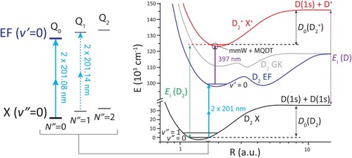
Table 1. Overview of the best previously determined dissociation energy (experiment and theory) and ionisation energy of ${\mathrm{D}}_2$, measured via the GK state, with the energy intervals required for the determination.

	Energy level interval	Value (cm${}^{-1}$)	Uncertainty (kHz)	Reference
(1)	$E_{\mathrm{I}}^{N=0}$(${\mathrm{D}}_2$)${}^{\mathrm{a}}=\left(4\right)-\left(5\right)+\left(6\right)$	124,745.393739(26)	780	[13]
(2)	$D_0^{N=0}$(${\mathrm{D}}_2$)${}^{\mathrm{a}}$ through GK	36,748.362282(26)	780	[13]
(3)	$D_0^{N=0}$(${\mathrm{D}}_2$)${}^{\mathrm{b}}$	36,748.362342(26)	780	[16]
(4)	$\mathrm{G}\mathrm{K}(v^{\prime }=1,N^{\prime }=2)\leftarrow \mathrm{X}(v^{″}=0,N^{″}=0)$ (${\mathrm{D}}_2$)${}^{\mathrm{a}}$	112,099.087712(15)	450	[13]
(5)	$\mathrm{G}\mathrm{K}(v^{\prime }=1,N^{\prime }=2)\leftarrow \mathrm{G}\mathrm{K}(v^{″}=0,N^{″}=2)$ (${\mathrm{D}}_2$)${}^{\mathrm{a}}$	333.038775(7)	210	[13]
(6)	${\mathrm{X}}^{+}(v^{+}=0,N^{+}=0)\leftarrow \mathrm{G}\mathrm{K}(v^{″}=0,N^{″}=2)$ (${\mathrm{D}}_2$)${}^{\mathrm{a}}$	12,979.344802(20)	600	[13]
(7)	$E_{\mathrm{I}}^{N=0}$(D)${}^{\mathrm{b}}$	109,708.61455294(17)	5	[22]
(8)	$E_{\mathrm{I}}^{N=0}$(${\mathrm{D}}_2^{+}$)${}^{\mathrm{b}}$	131,420.1976492(8)	24	[23]
(9)	$D_0^{N=1}$(${\mathrm{H}}_2$)${}^{\mathrm{a}}$ through EF	35,999.582834(11)	340	[12]
(10)	$D_0^{N=1}$(${\mathrm{H}}_2$)${}^{\mathrm{b}}$	35,999.582820(26)	780	[14]
(11)	$D_0^{N=0}$(${\mathrm{H}}_2$)${}^{\mathrm{c}}$ through GK	36,118.069605(31)	940	[17]
(12)	$D_0^{N=0}$(${\mathrm{H}}_2$)${}^{\mathrm{b}}$	36,118.069632(26)	780	[14]

Notes: In this table N indicates the rotational quantum number. The last part of the table also lists the most recent determinations of the dissociation energy for ortho- (N = 1) and para-${\mathrm{H}}_2$ (N = 0), measured through the EF and GK state respectively.

${}^{\mathrm{a}}$ experiment

${}^{\mathrm{b}}$ theory

${}^{\mathrm{c}}$ combination of theory and experiment

Figure 2. Ramsey-comb spectroscopy principle. The laser excitation is based on a pair of pulses that are separated in time by a macro-delay equal to an integer number N of the repetition period $T_{\mathrm{r}\mathrm{e}\mathrm{p}}$. For each macro-delay $N\times T_{\mathrm{r}\mathrm{e}\mathrm{p}}$, a scan of a micro-delay $\delta t$ is implemented by adjusting the repetition rate of the frequency comb laser at the ppb-level. The transition frequency can be extracted by a collective fit of the relative phase of all recorded Ramsey fringes. A longer maximal interpulse delay $\mathrm{\Delta }{t}_{\mathrm{m}\mathrm{a}\mathrm{x}}=N_{\mathrm{m}\mathrm{a}\mathrm{x}}{T}_{\mathrm{r}\mathrm{e}\mathrm{p}}$ results in a higher accuracy of the measured transition frequency and is ultimately limited by decoherence as shown in Figure 3.

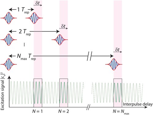
Figure 3. Example of a typical Ramsey-comb measurement in ${\mathrm{D}}_2$, for the extraction of the $\mathrm{E}\mathrm{F}(v^{\prime }=0,N^{\prime }=0)\leftarrow \mathrm{X}(v^{″}=0,N^{″}=0)$  transition frequency. Three fringes: $N=3$, 24 and 45 are recorded. The Ramsey fringe number N and interpulse delay $T_{\mathrm{r}\mathrm{e}\mathrm{p}}=1/f_{\mathrm{r}\mathrm{e}\mathrm{p}}$, set by the repetition rate $f_{\mathrm{r}\mathrm{e}\mathrm{p}}$ of the frequency comb, are scanned in a random order (top panel), and the data is then rearranged for further data analysis (bottom panel). The contrast and signal strength are high for short interpulse delays (87% at N = 3), and decrease for longer interpulse delays (43% at N = 45) due to the finite excited-state lifetime, the finite transit time of the molecules through the interaction zone and other sources of decoherence such as laser phase noise.

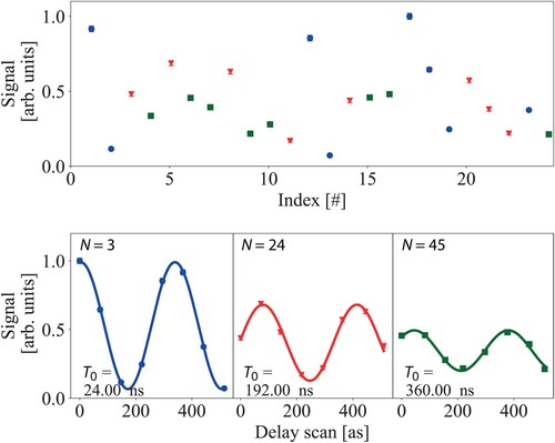
Figure 4. Schematic overview of the entire experimental setup. Two laser pulses from a NIR frequency comb are selectively amplified using a noncollinear optical parametric chirped-pulse amplifier (NOPCPA). The NOPCPA is driven by a pulsed pump laser, of which the repetition rate is synchronised to that of the NIR frequency comb. The pump laser produces high-intensity pulse pairs at 532 nm that are spatially and temporally overlapped with the two comb laser pulses in the beta barium borate (BBO) crystals of the NOPCPA. The resulting optical parametric amplification process leads to two NIR pulses of about 2.5 mJ (each) at the desired interpulse delay. These are then frequency-upconverted to perform the Ramsey-comb measurement in the vacuum setup on ${\mathrm{D}}_2$. Also shown is a phase measurement setup that monitors the phase influence of the NOPCPA, by combining light of the same frequency comb pulse before and after the NOPCPA.

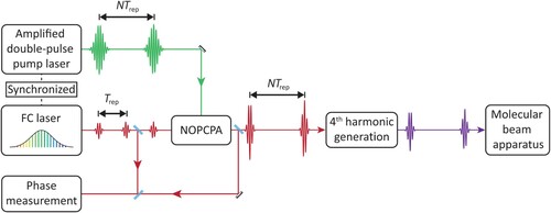
Figure 5. NIR frequency comb and pump synchronisation setup. The NIR frequency comb is optically locked to a narrow-linewidth cw laser referenced to an ultrastable optical reference cavity. The carrier-envelope offset frequency of the comb, $f_{\mathrm{c}\mathrm{e}\mathrm{o}}$, is locked to the 50 MHz output of a Direct Digital Synthesizer (DDS) referenced to a caesium atomic clock. The repetition rate of the pump laser oscillator (125 MHz) is locked to half the repetition rate of the frequency comb (250 MHz) to ensure timing overlap of the pulses from the systems in the NOPCPA, where the frequency comb pulses are amplified. Both ${\mathrm{f}}_{\mathrm{r}\mathrm{e}\mathrm{p}}$ and $f_{\mathrm{c}\mathrm{e}\mathrm{o}}$ are recorded during the Ramsey-comb measurements. The fundamental wavelength of the comb is shifted from 1550 nm to 1600 nm with a Raman-shifting fibre, after which the entire spectrum is frequency doubled to 804.32 nm, required for further upconversion to 201.08 nm for ${\mathrm{D}}_2$ spectroscopy. A 4f-grating stretcher with spectral filtering selects the central wavelength and bandwidth, and sets a frequency comb pulse duration of 7 ps, which is optimal for NOPCPA amplification with 48 ps pump pulses. Half-wave plates (HWP) enable optimisation of the polarisation for the gratings and for the single-mode polarisation maintaining fibre going to the NOPCPA.

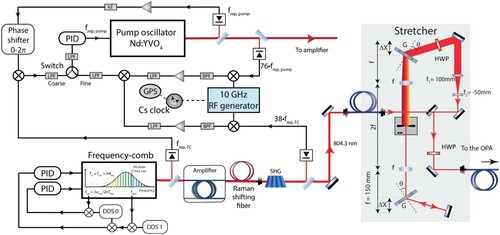
Figure 6. Phase measurement setup for the monitoring of NOPCPA-induced differential amplification phase shifts. The phase measurement is based on spectral interferometry. Part of the amplified frequency comb pulses are combined with their corresponding reference frequency comb pulses in a single-mode fibre to ensure perfect spatial overlap. Two Pockels cells (PC1 and PC2), in combination with polarisation beam splitters, suppress the non-amplified background pulses. A third Pockels cell (PC3) selects one of the amplified/non-amplified pulse combinations and displaces it vertically compared to the other pulse combination. The pulses are then sent onto a gold diffraction grating and are imaged onto an image intensifier ('Cricket' from Photonis) and CMOS camera (Manta G-235B from Allied Vision) to detect the interference pattern associated with each pulse.

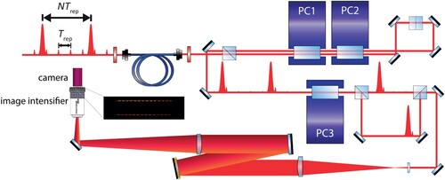
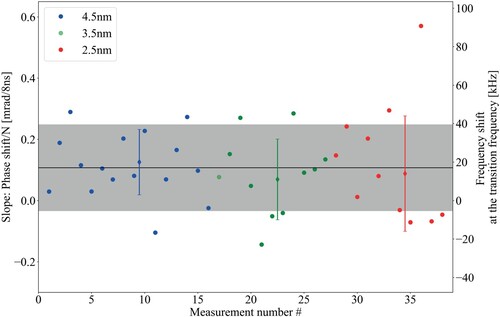
Figure 7. Typical differential phase measurement of the amplified frequency comb pulses, at a pulse bandwidth of 4.5 nm. A linear fit is performed to extract the phase shift with respect to the interpulse delay. This example measurement shows a time delay-dependent slope in relative phase shift of 0.103(0.071) mrad per 8 ns ($\mathrm{\Delta }N=1$), which results in a frequency shift of 16.4(11.3) kHz on the observed transition frequency in the DUV.

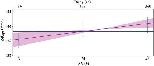
Figure 8. Deep-UV laser excitation and detection setup for Doppler-free Ramsey-comb spectroscopy. The NOPCPA-amplified NIR frequency comb pulses are frequency-upconverted from 804.32 to 201.08 nm in three BBO crystals. The DUV pulses are then split in two different paths by a metallic beam splitter (BS) and recombined onto a cold and slow ${\mathrm{D}}_2$ molecular beam in a Doppler-free counter-propagating excitation geometry (both paths towards the molecular beam are in reality equal in length). A 355 nm laser pulse selectively ionises those molecules that have been excited successfully to the EF state, 5 ns after the second Ramsey-comb excitation pulse. The resulting ions are then sent through a time-of-flight mass spectrometer (with a pulsed field that is switched on just after the ionisation pulse to minimise dc-Stark effects) and then detected with an electron multiplier (EM). The beam splitter also forms the exit port of a Sagnac interferometer (SI), which is used to monitor the relative alignment of the two counterpropagating beams. Sk1 is a skimmer with 3 mm opening, and Sk2 has an opening of 8 mm.

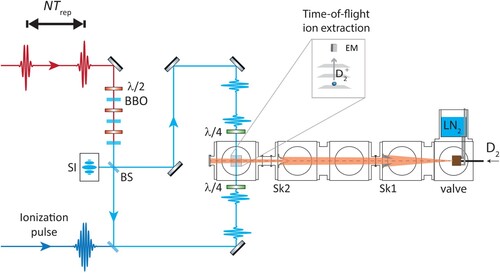
Table 2. Determination of the $\mathrm{E}\mathrm{F}(v^{\prime }=0,N^{\prime }=0)\leftarrow \mathrm{X}(v^{″}=0,N^{″}=0)$  transition frequency in molecular deuterium, including all corrections and uncertainties.

	Value or correction (kHz)	Uncertainty (kHz)
First-order Doppler-free and
amplifier-phase-shift corrected frequency	2,981,779,227,585	13
Corrections
Second-order Doppler	−9	2
ac-Stark shift	9	14
Phase measurement setup offset	−6	2
Zeeman shift	0	1
Cs clock	−1	0.15
dc-Stark shift	0	1
Total	2,981,779,227,578	19

Figure 9. Example of an extrapolation to zero velocity of the first-order residual Doppler shift on the $\mathrm{E}\mathrm{F}(v^{\prime }=0,N^{\prime }=0)\leftarrow \mathrm{X}(v^{″}=0,N^{″}=0)$  $Q_0$ transition in ${\mathrm{D}}_2$. The extrapolation is based on two sets of 3 measurements, one set performed with pure ${\mathrm{D}}_2$ gas with a mean velocity of 999(29) m/s, and the other with a 2D${}_2$:3 Ne mixture that has a mean ${\mathrm{D}}_2$ velocity of 571(13) m/s.

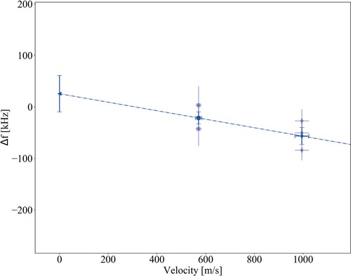
Figure 10. Example of NOPCPA-induced amplification phase shift measurements as measured before (left of the vertical line) and after (right of the vertical line) the Ramsey-comb measurements used for the determination of the first-order Doppler-free transition frequency. For the phase measurement, the same micro-delays and inter-pulse delays were used as during the spectroscopy. The averaged frequency shift of −29.7(15.3) kHz, calculated from these measurements, is used to correct the first-order Doppler-free transition frequency obtained on that day. The error bar from the fit of the individual phase shift measurements is not plotted because the observed variations are several times larger due to external influences. Therefore the uncertainty on the calculated averaged frequency shift correction is directly derived from the variation of the phase measurements with equal weight for all data points.

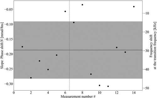
Figure 11. First-order Doppler-free transition frequency determination for each measurement day of the $\mathrm{E}\mathrm{F}(v^{\prime }=0,N^{\prime }=0)\leftarrow \mathrm{X}(v^{″}=0,N^{″}=0)$  $Q_0$ transition in ${\mathrm{D}}_2$. The frequency is given relative to an offset frequency of −2 MHz with respect to the previously determined value [24]. The first-order Doppler-free frequency is corrected for the amplifier phase shift and averaged over 5 days to reach a statistical accuracy of 13 kHz (shown by the pink band as the weighted standard error). The dotted line shows the weighted standard deviation at 30 kHz. During the measurement campaign, the nonlinear crystals for DUV generation deteriorated, resulting in reduced measurement statistics and making it progressively harder to continue the experiment. In particular, during the last measurement day, the signal strength and contrast were much lower.

Figure 12. (a) Identification of the ${\mathrm{D}}_2$ transition by an overview scan of Ramsey fringes obtained for different pulse pair combinations N, associated with the macro-delay $\mathrm{\Delta }t=N\times T_{\mathrm{r}\mathrm{e}\mathrm{p}}$. The maximum interpulse delay recorded is $\mathrm{\Delta }t=360$ ns, corresponding to N = 45. The measurement data are shown in blue. The red fit is performed on each Ramsey fringe while the green fit uses all fringes with an exponentially decaying amplitude to account for the contrast loss at higher N. (b) The Fourier transformation of 35 Ramsey-fringes. An interpulse delay spacing of $\mathrm{\Delta }N=3$ between the Ramsey-fringes is used to discriminate between all possible values of the transition frequencies modulo $f_{\mathrm{r}\mathrm{e}\mathrm{p}}/\mathrm{\Delta }N$ (41.7 MHz in this case). The blue curve corresponds to the Fourier transform of the data while the red one corresponds to the Fourier transform of the fit. The difference is shown by the violet curve. The vertical lines represent the values of the corresponding transition frequency determined in [24]. The corresponding uncertainties (1σ) are shown by the dashed lines. The Fourier peak coincides with the previous $Q_0$.

Figure 13. Self-reference phase measurements, used to quantify the systematic error induced by the phase measurement setup itself. The effective frequency shift due to the offset from zero is equivalent to 6(2) kHz in the DUV, and must be subtracted from the determined transition frequency.

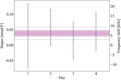
Figure 14. Determination of the ac-Stark shift on the transition frequency by evaluating the shift of the transition frequency at 54(3) $\mu$J /pulse (at which the first-order Doppler-free measurements were performed) based on a linear interpolation of transition frequencies at 23(1) $\mu$J/pulse and 63(3) $\mu$J /pulse. These measurements were performed over 4 days, where each point in the graph is based on at least three sets of ac-Stark measurements, that in turn are each based on 3 Ramsey-comb measurements at both low and high pulse energy. The weighted average over all measurements results in an ac-Stark shift of −9(14) kHz from the 201 nm excitation pulses, with the standard error shown by the pink band. The pink dotted line shows the weighted standard deviation of 59 kHz, and the different colours of the data points represent different days.

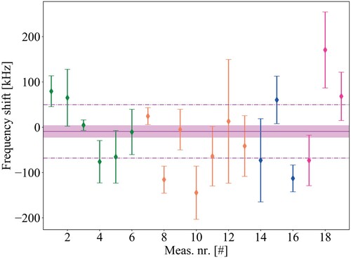
Figure 15. The dc Stark effect on the $\mathrm{E}\mathrm{F}(v^{\prime }=0,N^{\prime }=0)\leftarrow \mathrm{X}(v^{″}=0,N^{″}=0)$  $Q_0$ transition in ${\mathrm{D}}_2$ due to a residual electric field of -1.2 V/cm in the interaction zone. This is determined based on a comparison with measurements at high electric field (29.4  V/cm), and it is consistent with zero. The violet band represents the weighted standard error equal to 1 kHz while the dashed line shows the weighted standard deviation of 2 kHz.

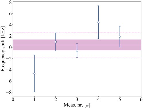
Figure 16. Experimental evaluation of the Zeeman effect on the $\mathrm{E}\mathrm{F}(v^{\prime }=0,N^{\prime }=0)\leftarrow \mathrm{X}(v^{″}=0,N^{″}=0)$  $Q_0$ transition in ${\mathrm{D}}_2$, performed by varying the magnetic field (applied perpendicularly to the polarisation axis of the DUV beams) between 0 and 6 G. A shift of 2.1(2.3) kHz/G was measured. This results in an effective shift of 0(1) kHz, consistent with zero, for our Ramsey-comb measurements during which the magnetic field is compensated to within 0.4 G at the interaction zone.

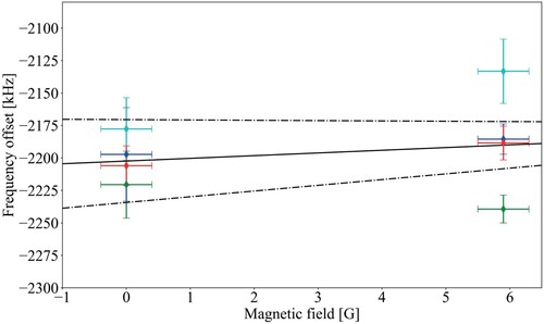
Figure A1. Comparison of the linear relative phase shifts for different bandwidths of the amplified FC laser. The average of all measurements is shown as the horizontal black line and its standard deviation by the grey band. The individual averages and standard deviations for each probed bandwidth are shown in the respective colour. No significant difference in the spread of slopes could be observed for bandwidths ranging between 2.5 and 4.5 nm.

J. Hussels, N. Hölsch, C.F. Cheng, E.J. Salumbides, H.L. Bethlem, K.S.E. Eikema, C. Jungen, M. Beyer, F. Merkt and W. Ubachs, Phys. Rev. A. 105 (2), 022820 (2022). doi:10.1103/PhysRevA.105.022820

 Web of Science ®Google Scholar

M. Puchalski, J. Komasa, A. Spyszkiewicz and K. Pachucki, Phys. Rev. A. 100 (2), 020503 (2019). doi:10.1103/PhysRevA.100.020503

 Google Scholar

V.A. Yerokhin, K. Pachucki and V. Patkóš, Ann. Phys. 531 (5), 1800324 (2019). doi:10.1002/andp.v531.5

 Google Scholar

V.I. Korobov, L. Hilico and J.P. Karr, Phys. Rev. Lett. 118 (23), 233001 (2017). doi:10.1103/PhysRevLett.118.233001

 PubMedGoogle Scholar

N. Hölsch, M. Beyer, E.J. Salumbides, K.S.E. Eikema, W. Ubachs, C. Jungen and F. Merkt, Phys. Rev. Lett. 122 (10), 103002 (2019). doi:10.1103/PhysRevLett.122.103002

 PubMed Web of Science ®Google Scholar

M. Puchalski, J. Komasa, P. Czachorowski and K. Pachucki, Phys. Rev. Lett.122 (10), 103003 (2019). doi:10.1103/PhysRevLett.122.103003

 PubMed Web of Science ®Google Scholar

M. Beyer, N. Hölsch, J. Hussels, C.F. Cheng, E.J. Salumbides, K.S.E. Eikema, W. Ubachs, C. Jungen and F. Merkt, Phys. Rev. Lett. 123 (16), 163002 (2019). doi:10.1103/PhysRevLett.123.163002

 PubMed Web of Science ®Google Scholar

S. Hannemann, E.J. Salumbides, S. Witte, R.T. Zinkstok, E.J. van Duijn, K.S.E. Eikema and W. Ubachs, Phys. Rev. A. 74 (6), 062514 (2006). doi:10.1103/PhysRevA.74.062514

 Google Scholar