Extraction of spin-averaged rovibrational transition frequencies in HD⁺ for the determination of fundamental constants

Figures & data

Table 1. Theoretical hyperfine coefficients of rovibrational states of ${\mathrm{HD}}^{+}$ involved in high-precision measurements, in kHz. Missing numbers in the first line imply a zero value. The values of $E_4/h$, $E_5/h$ ($E_1/h$, $E_6/h$, $E_7/h$) were calculated in Ref. [27] (Ref. [33]). Those of $E_2/h$, $E_3/h$, $E_8/h$, and $E_9/h$ are taken from [26]. The value of $E_9/h$ has been updated using the latest determination of the deuteron's quadrupole moment [34].

$(v,L)$	$E_1/h$	$E_2/h$	$E_3/h$	$E_4/h$	$E_5/h$	$E_6/h$	$E_7/h$	$E_8/h$	$E_9/h$
$(0,0)$				925,394.159(860)	142,287.556(84)
$(0,1)$	31,985.417(116)	$-31.345(8)$	$-4.809(1)$	924,567.718(859)	142,160.670(84)	8611.299(18)	1321.796(3)	$-3.057(1)$	5.660(1)
$(1,1)$	30,280.736(109)	$-30.463(8)$	$-4.664(1)$	903,366.501(839)	138,910.266(82)	8136.858(17)	1248.963(3)	$-2.945(1)$	5.653(1)
$(0,3)$	31,628.097(114)	$-30.832(8)$	$-4.733(1)$	920,479.981(855)	141,533.075(83)	948.542(2)	145.597	$-0.335$	0.613
$(9,3)$	18,270.853(62)	$-21.304(6)$	$-3.225(1)$	775,706.122(721)	119,431.933(73)	538.999(1)	82.726	$-0.219$	0.501

Table 2. Theoretical hyperfine shifts (column 3) and sensitivity coefficients (columns 4-12) for all the levels involved in high-precision measurements. Missing numbers for the $(v,L)=(0,0)$ state imply a zero value. The uncertainties of the hyperfine shifts are calculated assuming no correlation between $\delta E_k(v,L)$ and $\delta E_k(v^{\prime },L^{\prime })$ for $k\ne 4,5$, which provides an upper bound of the uncertainty.

$(v,L)$	$(F,S,J)$	$E_{\mathrm{hfs}}/h$ (kHz)	${\gamma }_1$	${\gamma }_2$	${\gamma }_3$	${\gamma }_4$	${\gamma }_5$	${\gamma }_6$	${\gamma }_7$	${\gamma }_8$	${\gamma }_9$
$(0,0)$	$(0,1,1)$	$-\mathrm{705,735.655}(639)$				$-0.7367$	$-0.1688$
	$(1,0,0)$	89,060.984(197)				0.2500	$-1.0000$
	$(1,1,1)$	171,894.797(194)				0.2367	$-0.3312$
	$(1,2,2)$	302,492.318(235)				0.2500	0.5000
$(0,1)$	$(0,1,2)$	$-\mathrm{707,870.694}(637)$	$-0.1070$	0.1110	0.9953	$-0.7338$	$-0.1845$	0.0100	0.1434	$-0.1572$	$-0.4930$
	$(1,0,1)$	79,986.308(204)	$-0.4286$	$-0.3861$	0.6539	0.2494	$-0.9084$	$-1.0279$	0.8343	0.7206	$-0.5019$
	$(1,1,2)$	183,682.795(196)	0.3319	0.1539	0.5142	0.2341	$-0.3152$	0.2555	$-0.5821$	$-0.4019$	0.2287
	$(1,2,1)$	269,283.177(241)	$-0.5693$	$-0.5592$	$-1.7183$	0.2500	0.4251	0.0392	$-3.3471$	$-3.2839$	$-2.9444$
	$(1,2,3)$	312,567.273(242)	0.5000	0.5000	1.0000	0.2500	0.5000	$-0.5000$	$-1.0000$	$-1.0000$	$-0.5000$
	$(1,2,2)$	314,228.466(238)	$-0.2249$	$-0.2649$	$-0.5096$	0.2497	0.4997	1.7345	3.4387	3.5591	1.7643
$(1,1)$	$(1,2,1)$	263,806.300(235)	$-0.5753$	$-0.5654$	$-1.7152$	0.2500	0.4296	$-0.0105$	$-3.3687$	$-3.3063$	$-2.9087$
	$(1,2,3)$	305,099.957(236)	0.5000	0.5000	1.0000	0.2500	0.5000	$-0.5000$	$-1.0000$	$-1.0000$	$-0.5000$
$(0,3)$	$(0,1,4)$	$-\mathrm{711,832.144}(631)$	$-0.4142$	0.4242	2.9867	$-0.7267$	$-0.2156$	0.2750	3.0796	$-3.3289$	$-7.4000$
	$(1,2,5)$	338,970.635(290)	1.5000	1.5000	3.0000	0.2500	0.5000	$-7.5000$	$-15.0000$	$-15.0000$	$-7.5000$
$(9,3)$	$(0,1,4)$	$-\mathrm{596,833.613}(533)$	$-0.3590$	0.3727	2.9847	$-0.7303$	$-0.2017$	0.1934	2.4743	$-2.7221$	$-7.3853$
	$(1,2,5)$	275,723.281(219)	1.5000	1.5000	3.0000	0.2500	0.5000	$-7.5000$	$-15.0000$	$-15.0000$	$-7.5000$

Table 3. Experimentally determined transition frequencies, $f^{\exp }[(v,L,a)\to (v^{\prime },L^{\prime },a^{\prime })]$ (where $a=(F,S,J)$ and $a^{\prime }=(F^{\prime },S^{\prime },J^{\prime })$), of various hyperfine components used in the adjustment of the spin-averaged transition frequencies (Section 4). The alternate labels for the hyperfine components in column 6 are those used in the original references (column 7).

$(v,L)\to (v^{\prime },L^{\prime })$	Label	$(F,S,J)$	$(F^{\prime },S^{\prime },J^{\prime })$	$f^{\exp }[(v,L,a)\to (v^{\prime },L^{\prime },a^{\prime })]$ (kHz)	Alt. label	Ref.
$(0,0)\to (0,1)$	A1	(1,2,2)	(1,2,1)	1,314,892,544.276(40)	12	[14]
	A2	(1,0,0)	(1,0,1)	1,314,916,678.487(64)	14
	A3	(0,1,1)	(0,1,2)	1,314,923,618.028(17)	16
	A4	(1,2,2)	(1,2,3)	1,314,935,827.695(37)	19
	A5	(1,2,2)	(1,2,2)	1,314,937,488.614(60)	20
	A6	(1,1,1)	(1,1,2)	1,314,937,540.762(46)	21
$(0,0)\to (1,1)$	A7	(1,2,2)	(1,2,1)	58,605,013,478.03(19)	12	[16]
	A8	(1,2,2)	(1,2,3)	58,605,054,772.08(26)	16
$(0,3)\to (9,3)$	A9	(0,1,4)	(0,1,4)	415,265,040,503.57(59)	F = 0	[15]
	A10	(1,2,5)	(1,2,5)	415,264,862,249.16(66)	F = 1

Table 4. Input data for the additive energy corrections to account for the theoretical uncertainties of hyperfine interaction coefficients.

	Input datum	Value (kHz)		Input datum	Value (kHz)
B1	$\delta E_4(0,0)/h$	0.000(860)	B12	$\delta E_9(1,1)/h$	0.00000(55)
B2	$\delta E_5(0,0)/h$	0.000(84)	B13	$\delta E_1(0,3)/h$	0.000(114)
B3	$\delta E_1(0,1)/h$	0.000(116)	B14	$\delta E_2(0,3)/h$	0.0000(82)
B4	$\delta E_2(0,1)/h$	0.0000(83)	B15	$\delta E_6(0,3)/h$	0.0000(20)
B5	$\delta E_6(0,1)/h$	0.000(18)	B16	$\delta E_8(0,3)/h$	0.000000(89)
B6	$\delta E_8(0,1)/h$	0.00000(81)	B17	$\delta E_9(0,3)/h$	0.000000(60)
B7	$\delta E_9(0,1)/h$	0.00000(55)	B18	$\delta E_1(9,3)/h$	0.000(62)
B8	$\delta E_1(1,1)/h$	0.000(109)	B19	$\delta E_2(9,3)/h$	0.0000(57)
B9	$\delta E_2(1,1)/h$	0.0000(81)	B20	$\delta E_6(9,3)/h$	0.0000(12)
B10	$\delta E_6(1,1)/h$	0.000(17)	B21	$\delta E_8(9,3)/h$	0.000000(58)
B11	$\delta E_8(1,1)/h$	0.00000(78)	B22	$\delta E_9(9,3)/h$	0.000000(49)

Table 5. Spin-averaged transition frequencies $f_{\mathrm{SA}}$ (in kHz). Previous determinations from the original publications [14–16] are given in the first line. The results of the least-squares adjustment performed in the present work are given in line 2. These results were obtained with an expansion factor $\eta =1$ (i.e. no expansion factor applied). The spin-averaged frequencies in line 3 are obtained by applying an expansion factor $\eta =3.56$ to the uncertainties of all (experimental and theoretical) input data. Finally, line 4 shows the frequencies for $\eta =3.56$ and including the hyperfine-correlation-induced uncertainty; see text for details. The frequencies on line 4 are our recommended values.

	$(0,0)\to (0,1)$	$(0,0)\to (1,1)$	$(0,3)\to (9,3)$
$f_{\mathrm{SA}}$ (previous)	1,314,925,752.910(17)	58,605,052,164.24(86)	415,264,925,500.5(1.2)
$f_{\mathrm{SA}}$ ($\eta =1$)	1,314,925,752.978(14)	58,605,052,164.14(16)	415,264,925,501.3(0.4)
$f_{\mathrm{SA}}$ ($\eta =3.56$)	1,314,925,752.978(48)	58,605,052,164.14(55)	415,264,925,501.3(1.6)
$f_{\mathrm{SA}}$ ($\eta =3.56$ and corr. ind. unc.)	1,314,925,752.978(48)	58,605,052,164.14(56)	415,264,925,501.3(1.6)

Table 6. Reference theoretical values and sensitivity coefficients of ${\mathrm{HD}}^{+}$ transition frequencies. The theoretical frequencies are calculated using 2018 CODATA values of $A_{\mathrm{r}}(\mathrm{e})$, $A_{\mathrm{r}}(\mathrm{p})$, $A_{\mathrm{r}}(\mathrm{d})$, $c{R}_{\mathrm{\infty }}$, $r_{\mathrm{p}}$, $r_{\mathrm{d}}$, and α. The sensitivity coefficient for the Rydberg constant ${\beta }_{c{R}_{\mathrm{\infty }}}$ is dimensionless. u stands for the relative atomic mass unit.

	$f_{\mathrm{SA}}^{\mathrm{theor}}$		${\eta }_{r_{\mathrm{p}}}$	${\eta }_{r_{\mathrm{d}}}$
Transition	(kHz)	${\beta }_{c{R}_{\mathrm{\infty }}}$	(kHz.fm${}^{-2}$)	(kHz.fm${}^{-2}$)
$(0,0)\to (0,1)$	1,314,925,752.929	$3.9969[-04]$	$-9.0991[-01]$	$-9.0991[-01]$
$(0,0)\to (1,1)$	58,605,052,163.88	$1.7814[-02]$	$-2.4253[+01]$	$-2.4220[+01]$
$(0,3)\to (9,3)$	415,264,925,502.7	$1.2623[-01]$	$-1.5940[+02]$	$-1.5850[+02]$
	${\beta }_{{\lambda }_{\mathrm{pd}}}$	${\beta }_{{\lambda }_{\mathrm{d}}}$	${\beta }_{A_{\mathrm{r}}(\mathrm{e})}$	${\beta }_{A_{\mathrm{r}}(\mathrm{p})}$	${\beta }_{A_{\mathrm{r}}(\mathrm{d})}$
Transition	(kHz)	(kHz)	(kHz.u${}^{-1}$)	(kHz.u${}^{-1}$)	(kHz.u${}^{-1}$)
$(0,0)\to (0,1)$	$-1.0601[+06]$	$-3.2126[+01]$	$2.3653[+12]$	$-8.5857[+08]$	$-2.1492[+08]$
$(0,0)\to (1,1)$	$-2.3201[+07]$	$-7.0874[+02]$	$5.1767[+13]$	$-1.8790[+10]$	$-4.7036[+09]$
$(0,3)\to (9,3)$	$-1.2580[+08]$	$-3.9569[+03]$	$2.6664[+14]$	$-9.6785[+10]$	$-2.4227[+10]$

Figure 1. Normalised residuals of the 32 input data for the adjustment of spin-averaged transition frequencies. Labels Ai and Bi follow those defined in Tables 3 and 4.

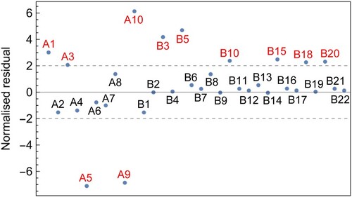
Table 7. Input data for the adjustments discussed in Section 5. Entries C1 and C5–C7 also serve as reference values in Equations (8(8) $\begin{array}{rl}& f_{\mathrm{SA}}[(v,L)\to (v^{\prime },L^{\prime })]\\ & \doteq f_{\mathrm{SA}}^{\mathrm{th}}[(v,L)\to (v^{\prime },L^{\prime })]+\delta f^{\mathrm{th}}(v,L,v^{\prime },L^{\prime })\\ & +{\beta }_{R_{\mathrm{\infty }}}c(R_{\mathrm{\infty }}-R_{\mathrm{\infty }0})+{\eta }_{r_{\mathrm{p}}}(r_{\mathrm{p}}^2-r_{\mathrm{p}0}^2)\\ & +{\eta }_{r_{\mathrm{d}}}(r_{\mathrm{d}}^2-r_{\mathrm{d}0}^2)+{\beta }_{{\lambda }_{\mathrm{pd}}}({\lambda }_{\mathrm{pd}}-{\lambda }_{\mathrm{pd}0})\\ & +{\beta }_{{\lambda }_{\mathrm{d}}}({\lambda }_{\mathrm{d}}-{\lambda }_{\mathrm{d}0}).\end{array}$(8) ) and (14(14) $\begin{array}{rl}& f_{\mathrm{SA}}[(v,L)\to (v^{\prime },L^{\prime })]\\ & \doteq f_{\mathrm{SA}}^{\mathrm{th}}[(v,L)\to (v^{\prime },L^{\prime })]+\delta f(v,L,v^{\prime },L^{\prime })\\ & +{\beta }_{R_{\mathrm{\infty }}}c(R_{\mathrm{\infty }}-R_{\mathrm{\infty }0})+{\eta }_{r_{\mathrm{p}}}(r_{\mathrm{p}}^2-r_{\mathrm{p}0}^2)\\ & +{\eta }_{r_{\mathrm{d}}}(r_{\mathrm{d}}^2-r_{\mathrm{d}0}^2)\\ & +{\beta }_{A_{\mathrm{r}}(\mathrm{e})}(A_{\mathrm{r}}(\mathrm{e})-A_{\mathrm{r}}(\mathrm{e}{)}_0)\\ & +{\beta }_{A_{\mathrm{r}}(\mathrm{p})}(A_{\mathrm{r}}(\mathrm{p})-A_{\mathrm{r}}(\mathrm{p}{)}_0)\\ & +{\beta }_{A_{\mathrm{r}}(\mathrm{d})}(A_{\mathrm{r}}(\mathrm{d}))-A_{\mathrm{r}}(\mathrm{d}{)}_0).\end{array}$(14) ).

Label	Input datum	Value	Rel. uncertainty	Reference
A1	$f_{\mathrm{SA}}[(0,0)\to (0,1)]$	1,314,925,752.978(48) kHz	$3.7\times {10}^{-11}$	This work
A2	$f_{\mathrm{SA}}[(0,0)\to (1,1)]$	58,605,052,164.14(56) kHz	$9.6\times {10}^{-12}$	This work
A3	$f_{\mathrm{SA}}[(0,3)\to (9,3)]$	415,264,925,501.3(1.6) kHz	$3.9\times {10}^{-12}$	This work
B1	$\delta f(0,0,0,1)$	0.000(19) kHz		[19]
B2	$\delta f(0,0,1,1)$	0.00(49) kHz		[19]
B3	$\delta f(0,3,9,3)$	0.0(3.2) kHz		[19]
C1	$A_{\mathrm{r}}(\mathrm{e})$ (CODATA 2018)	5.48579909065(16)$\times {10}^{-4}$ u	$2.9\times {10}^{-11}$	[1]
C2	$A_{\mathrm{r}}(\mathrm{d})$ (AMDC 2020)	2.013553212537(15) u	$7.5\times {10}^{-12}$	[36]
C3	$A_{\mathrm{r}}(\mathrm{p})$ (AMDC 2020)	1.007276466587(14) u	$1.4\times {10}^{-11}$	[36]
C4	$m_{\mathrm{d}}/m_{\mathrm{p}}$ (Fink 2021)	1.999007501272(9)	$4.5\times {10}^{-12}$	[7]
C5	$c{R}_{\mathrm{\infty }}$ (CODATA 2018)	3,289,841,960,250.8(6.4) kHz	$1.9\times {10}^{-12}$	[1]
C6	$r_{\mathrm{p}}$ (CODATA 2018)	0.8414(19) fm	$2.2\times {10}^{-3}$	[1]
C7	$r_{\mathrm{d}}$ (CODATA 2018)	2.12799(74) fm	$3.5\times {10}^{-4}$	[1]

Table 8. Values of all nonzero correlation coefficients in the input data of Table 7.

Correlation coefficients
$r(\mathrm{A}1,\mathrm{A}2)=0.00036$	$r(\mathrm{A}1,\mathrm{A}3)=0.00644$	$r(\mathrm{A}2,\mathrm{A}3)=0.00741$	$r(\mathrm{B}1,\mathrm{B}2)=0.99570$
$r(\mathrm{B}1,\mathrm{B}3)=0.95733$	$r(\mathrm{B}2,\mathrm{B}3)=0.97998$	$r(\mathrm{C}1,\mathrm{C}5)=0.00704$	$r(\mathrm{C}1,\mathrm{C}6)=-0.00133$
$r(\mathrm{C}1,\mathrm{C}7)=0.00317$	$r(\mathrm{C}2,\mathrm{C}3)=0.31986$	$r(\mathrm{C}5,\mathrm{C}6)=0.88592$	$r(\mathrm{C}5,\mathrm{C}7)=0.90366$
$r(\mathrm{C}6,\mathrm{C}7)=0.99165$

Table 9. Adjustment results. $u_{\mathrm{r}}$ stands for relative uncertainty.

Adjustment	Input data	Adjusted value	$u_{\mathrm{r}}$ (${10}^{-11}$)
1	C1–C4	${\lambda }_{\mathrm{pd}}=\mathrm{1,223.899228646}(37)$	3.0
2	A,B,C5–C7	${\lambda }_{\mathrm{pd}}=\mathrm{1,223.899228719}(26)$	2.1
1	C1–C4	${\lambda }_{\mathrm{p}}=\mathrm{1,836.152673353}(56)$	3.0
3	All	${\lambda }_{\mathrm{p}}=\mathrm{1,836.152673423}(33)$	1.8
3	All	$A_{\mathrm{r}}(\mathrm{e})=5.48579909046(10)\times {10}^{-4}$ u	1.8

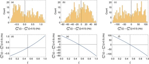
Figure A1. Distribution of correlation-induced shifts of spin-averaged frequencies obtained from a Monte-Carlo simulation consisting of 502 runs. Here the components of the vector $(r_1,r_2,r_6,r_8,r_9)$ are varied together as $(\xi ,\xi ,\xi ,\xi ,\xi )$; for example, $\xi =0.5$ stands for the vector $(0.5,0.5,0.5,0.5,0.5)$ (a) Distribution for the $(v,L)$: $(0,0)\to (0,1)$ transition. (b) Distribution for the $(v,L)$: $(0,0)\to (1,1)$ transition. (c) Distribution for the $(v,L)$: $(0,3)\to (9,3)$ transition. Dashed vertical lines indicate the mean value of the frequency distribution. (d) Frequency shift of the $(v,L)$: $(0,0)\to (0,1)$ transition versus ξ, with all components of the vector $(r_1,r_2,r_6,r_8,r_9)$ being varied together as $(\xi ,\xi ,\xi ,\xi ,\xi )$. (e) Same as (d), but for the $(v,L)$: $(0,0)\to (1,1)$ transition. (f) Same as (d), but for the $(v,L)$: $(0,3)\to (9,3)$ transition.

J.-Ph. Karr, M. Haidar, L. Hilico, Z.X. Zhong and V.I. Korobov, Phys. Rev. A 102, 052827 (2020). doi:10.1103/PhysRevA.102.052827

 Web of Science ®Google Scholar

M. Haidar, V.I. Korobov, L. Hilico and J.-Ph. Karr, Phys. Rev. A 106, 042815 (2022). doi:10.1103/PhysRevA.106.042815

 Web of Science ®Google Scholar

D. Bakalov, V.I. Korobov and S. Schiller, Phys. Rev. Lett. 97, 243001 (2006). doi:10.1103/PhysRevLett.97.243001

 PubMed Web of Science ®Google Scholar

M. Puchalski, J. Komasa and K. Pachucki, Phys. Rev. Lett. 125, 253001 (2020). doi:10.1103/PhysRevLett.125.253001

 PubMed Web of Science ®Google Scholar

S. Alighanbari, G.S. Giri, F.L. Constantin, V.I. Korobov and S. Schiller, Nature 581, 152–158 (2020). doi:10.1038/s41586-020-2261-5

 PubMed Web of Science ®Google Scholar

I.V. Kortunov, S. Alighanbari, M.G. Hansen, G.S. Giri, V.I. Korobov and S. Schiller, Nat. Phys. 17, 569–573 (2021). doi:10.1038/s41567-020-01150-7

 Web of Science ®Google Scholar

S. Patra, M. Germann, J.-Ph. Karr, M. Haidar, L. Hilico, V.I. Korobov, F.M.J. Cozijn, K.S.E. Eikema, W. Ubachs and J.C.J. Koelemeij, Science 369 (6508), 1238–1241 (2020). doi:10.1126/science.aba0453

 PubMed Web of Science ®Google Scholar

V.I. Korobov and J.-Ph. Karr, Phys. Rev. A 104, 032806 (2021). doi:10.1103/PhysRevA.104.032806

 Web of Science ®Google Scholar

E. Tiesinga, P.J. Mohr, D.B. Newell and B.N. Taylor, Rev. Mod. Phys. 93, 025010 (2021). doi:10.1103/RevModPhys.93.025010

 PubMed Web of Science ®Google Scholar

M. Wang, W.J. Huang, F.G. Kondev, G. Audi and S. Naimi, Chin. Phys. C 45 (3), 030003 (2021). doi:10.1088/1674-1137/abddaf

 Web of Science ®Google Scholar

D.J. Fink and E.G. Myers, Phys. Rev. Lett. 127, 243001 (2021). doi:10.1103/PhysRevLett.127.243001

 PubMed Web of Science ®Google Scholar