Why Bayesian Psychologists Should Change the Way They Use the Bayes Factor

Figures & data

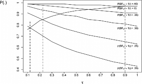
Figure 1. Probability of correctly preferring H₀ and H₁ as a function of τ for N = 100 based on the scaled information Bayes factor. Note that the optimal τ value according to Definition 1 can be found at the crossing of the line labeled P(BF₀₁ > 1|δ = 0) with the power curves P(BF₀₁ < 1|δ = ES) for ES ∈ {.20, .25, .30, .35, .40}. Vertical lines have been inserted in the figure at τ = .125, τ = .225, and τ = .90, to highlight crossings for effect sizes of .20, .25, and .40, respectively. The vertical line at the right also marks the optimal τ value according to Definition 2.

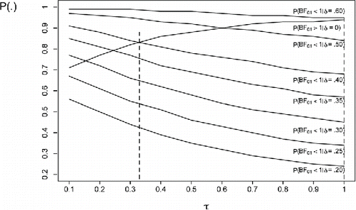
Figure 2. Probability of correctly preferring H₀ and H₁ as a function of τ for N = 36 based on the scaled information Bayes factor. Note that the optimal τ value according to Definition 1 can be found at the crossing of the line labeled P(BF₀₁ > 1|δ = 0) with the power curves P(BF₀₁ < 1|δ = ES) for ES ∈ {.20, .25, .30, .35, .40, .50, .60}. Vertical lines have been inserted in the figure at τ = .33, and τ = 1.0, to highlight crossings for effect sizes of .40 and .60, respectively. The vertical line at the right also marks the optimal τ value according to Definition 2.

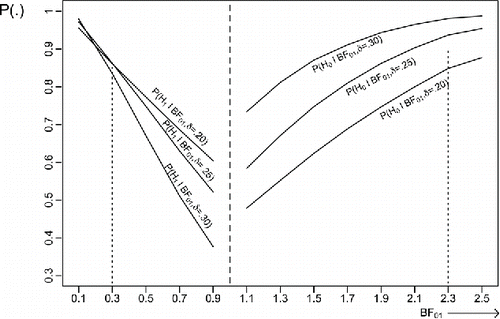
Figure 3. Conditional probabilities of preferring H₀ and H₁ given the observed size of the scaled information Bayes factor for N = 100 and τ = .225. The left hand side of the figure displays P(H₁|BF₀₁, δ = ES) for ES ∈ {.20, .25, .30} the right hand side of the figure displays P(H₀|BF₀₁, δ = ES) for ES ∈ {.20, .25, .30}. Vertical lines have been added to highlight the conditional probabilities at BF₀₁ = .3 and BF₀₁ = 2.3.