14,324
Views
106
CrossRef citations to date
0
Altmetric
Articles

An Introduction to Network Psychometrics: Relating Ising Network Models to Item Response Theory Models

Figures & data

Figure 1. A network of statistical models with the edges showing equivalence relation between the models subject to the constraints given on the edge labels. The edges are directed and originate from the more general model. The nodes refer to the extended Rasch model (E-RM), marginal Rasch model (M-RM), multidimensional two-parameter logistic model (MD-2PLM), Ising model (Ising), Curie-Weiss model (Curie-Weiss), and Logistic regression (LR).
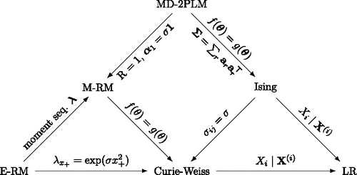
Figure 1. A network of statistical models with the edges showing equivalence relation between the models subject to the constraints given on the edge labels. The edges are directed and originate from the more general model. The nodes refer to the extended Rasch model (E-RM), marginal Rasch model (M-RM), multidimensional two-parameter logistic model (MD-2PLM), Ising model (Ising), Curie-Weiss model (Curie-Weiss), and Logistic regression (LR).

Figure 2. A square 3 × 3 lattice where the nodes (circles) refer to the upward “↑” or downward “↓” orientation of particles, and it is assumed that the particles only interact with their nearest neighbors (indicated with solid lines).
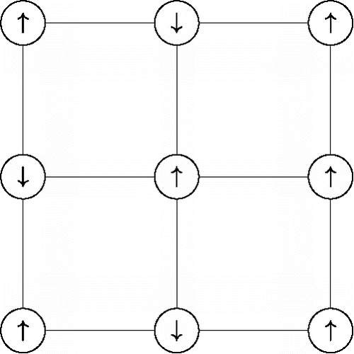
Figure 2. A square 3 × 3 lattice where the nodes (circles) refer to the upward “↑” or downward “↓” orientation of particles, and it is assumed that the particles only interact with their nearest neighbors (indicated with solid lines).

Figure 3. A network of five selected major depression (MD) and generalized anxiety disorder (GAD) symptoms that are taken from the fourth edition of the Diagnostic and Statistical Manual of Mental Disorders (DSM-IV; a complete version of this network is shown in Borsboom & Cramer, Citation2013). Irritability (I) and chronic worrying (C) are GAD symptoms, weight problems (W) and depressed mood (D) are MD symptoms, and sleep problems (S) is a symptom of both MD and GAD.
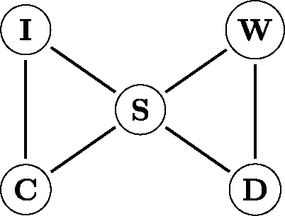
Figure 3. A network of five selected major depression (MD) and generalized anxiety disorder (GAD) symptoms that are taken from the fourth edition of the Diagnostic and Statistical Manual of Mental Disorders (DSM-IV; a complete version of this network is shown in Borsboom & Cramer, Citation2013). Irritability (I) and chronic worrying (C) are GAD symptoms, weight problems (W) and depressed mood (D) are MD symptoms, and sleep problems (S) is a symptom of both MD and GAD.

Figure 4. A common cause representation of the manifest relations between GAD and MD symptoms in .

Figure 4. A common cause representation of the manifest relations between GAD and MD symptoms in Figure 3.

Figure 5. A graphical representation of the Curie-Weiss network. The nodes (circles) refer to the upward “↑” and downward “↓” orientation of particles and each particle interacts with each other particle (solid lines).
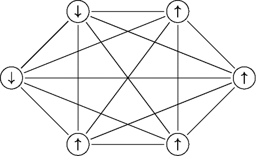
Figure 5. A graphical representation of the Curie-Weiss network. The nodes (circles) refer to the upward “↑” and downward “↓” orientation of particles and each particle interacts with each other particle (solid lines).

Figure 6. A graphical representation of the Rasch model. The observables (squares) refer to the upward “↑” and downward “↓” orientation of particles and each particle interacts with another particle only through the latent variable Θ.
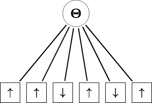
Figure 6. A graphical representation of the Rasch model. The observables (squares) refer to the upward “↑” and downward “↓” orientation of particles and each particle interacts with another particle only through the latent variable Θ.

Figure 7. Some instances of the structural model g(θ) for the n = 6 variable network. The solid line refers to the distribution with σ = 0.1 and the μi equally spaced between − 1 and + 1. The dashed line refers to the distribution with σ = 0.2 and the μi equally spaced between − 1 and + 1. The dotted line refers to the distribution with σ = 0.1 and the μi equally spaced between − 0.2 and + 1.
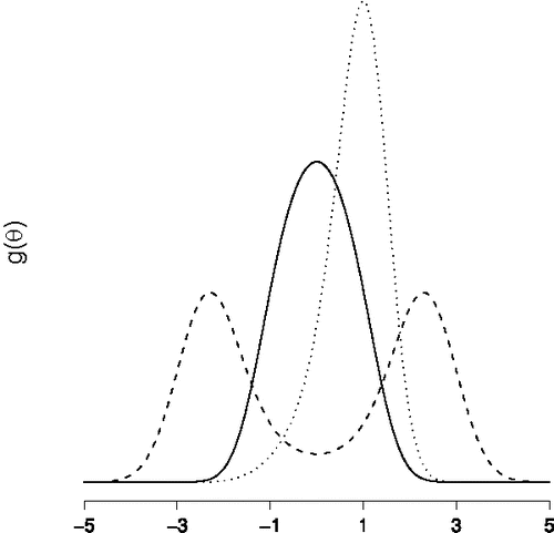
Figure 7. Some instances of the structural model g(θ) for the n = 6 variable network. The solid line refers to the distribution with σ = 0.1 and the μi equally spaced between − 1 and + 1. The dashed line refers to the distribution with σ = 0.2 and the μi equally spaced between − 1 and + 1. The dotted line refers to the distribution with σ = 0.1 and the μi equally spaced between − 0.2 and + 1.

Figure 8. The structural model g(θ) for in the absence of main effects, that is, μi = 0, and with an interaction strength σ = 0.075.
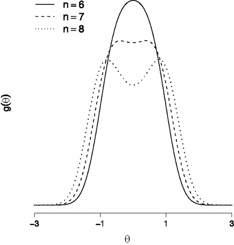
Figure 8. The structural model g(θ) for in the absence of main effects, that is, μi = 0, and with an interaction strength σ = 0.075.

Figure 9. The structural model gn(θ) for in the absence of main effects, that is, μi = 0, and with a scaled interaction strength σn = σ/n = 0.45/n. We have used σ = 0.45 since then the scaled structural model for n = 6 variables shown here is identical to the structural model for n = 6 variables in .
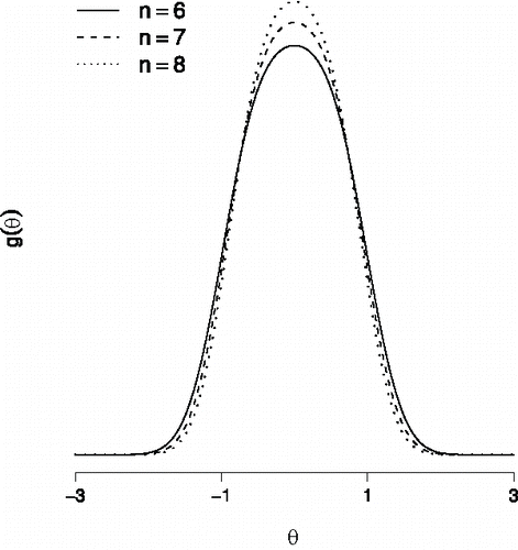
Figure 9. The structural model gn(θ) for in the absence of main effects, that is, μi = 0, and with a scaled interaction strength σn = σ/n = 0.45/n. We have used σ = 0.45 since then the scaled structural model for n = 6 variables shown here is identical to the structural model for n = 6 variables in Figure 8.

Figure 10. The first eigenvector corresponding to a decomposition of (left panel) and the first eigenvector corresponding to a decomposition of (right panel).
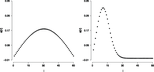
Figure 10. The first eigenvector corresponding to a decomposition of (left panel) and the first eigenvector corresponding to a decomposition of (right panel).

Figure 11. A graphical representation of the common effect model. The observables X are the collective cause of the effect Y.
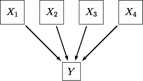
Figure 11. A graphical representation of the common effect model. The observables X are the collective cause of the effect Y.

Figure 12. The relation between conceptual, statistical, and causal models. Two different conceptual models (middle panel) that imply the same statistical observation model (top panel) can often still be teased apart using causal interventions (bottom panel).
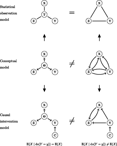
Figure 12. The relation between conceptual, statistical, and causal models. Two different conceptual models (middle panel) that imply the same statistical observation model (top panel) can often still be teased apart using causal interventions (bottom panel).

Figure 13. The left panel shows the average P-value obtained from KS-tests comparing the empirical CDF of plausible value with the Normal CDF for different values of the interaction strength σ. The right panel shows the true CDF of the latent variables (gray solid line), the estimated Normal CDF (black solid line), and the empirical CDF of plausible values (black dotted line) for σ = 0.04.
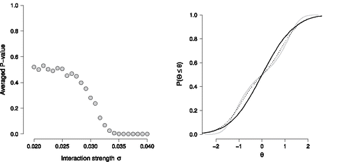
Figure 13. The left panel shows the average P-value obtained from KS-tests comparing the empirical CDF of plausible value with the Normal CDF for different values of the interaction strength σ. The right panel shows the true CDF of the latent variables (gray solid line), the estimated Normal CDF (black solid line), and the empirical CDF of plausible values (black dotted line) for σ = 0.04.
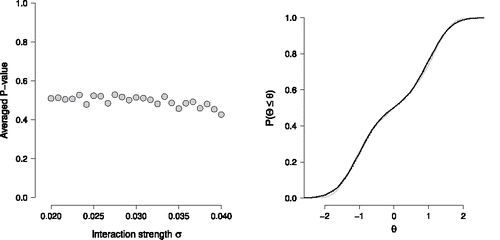
Figure 14. The left panel shows the average P-value obtained from KS-tests comparing the empirical CDF of plausible value with the estimated Normal mixture CDF for different values of the interaction strength σ. The right panel shows the true CDF of the latent variables (gray solid line), the estimated Normal mixture CDF (black solid line), and the empirical CDF of plausible values (black dotted line) for σ = 0.04.
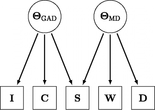
Figure 14. The left panel shows the average P-value obtained from KS-tests comparing the empirical CDF of plausible value with the estimated Normal mixture CDF for different values of the interaction strength σ. The right panel shows the true CDF of the latent variables (gray solid line), the estimated Normal mixture CDF (black solid line), and the empirical CDF of plausible values (black dotted line) for σ = 0.04.