6,760
Views
75
CrossRef citations to date
0
Altmetric
Articles

Modeling Nonstationary Emotion Dynamics in Dyads using a Time-Varying Vector-Autoregressive Model

, , , &

Figures & data

Figure 1. An example of a cubic regression spline basis for the model yt = βt + εt. The basis functions for the smooth curve βt of a cubic regression spline basis are shown. The first panel represents the data through which the smooth curve will be fitted. The knot locations are shown as vertical lines. The first basis function is defined as R1(t) = 1 and the other six basis functions (R2(t)–R7(t)) are spline-specific basis functions. Thus, with six knots there are seven basis functions in total. Just as in standard regression, all basis functions Ri(t) are weighed by multiplying them with their corresponding αi coefficients. These weighted basis functions are then summed up, resulting in the smooth curve (with CI) in the last panel at the bottom right where the black dots again represent the data.
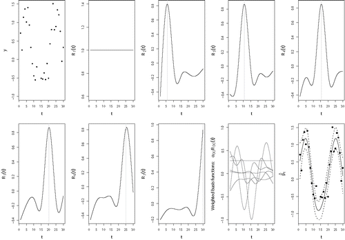
Figure 1. An example of a cubic regression spline basis for the model yt = βt + εt. The basis functions for the smooth curve βt of a cubic regression spline basis are shown. The first panel represents the data through which the smooth curve will be fitted. The knot locations are shown as vertical lines. The first basis function is defined as R1(t) = 1 and the other six basis functions (R2(t)–R7(t)) are spline-specific basis functions. Thus, with six knots there are seven basis functions in total. Just as in standard regression, all basis functions Ri(t) are weighed by multiplying them with their corresponding αi coefficients. These weighted basis functions are then summed up, resulting in the smooth curve (with CI) in the last panel at the bottom right where the black dots again represent the data.
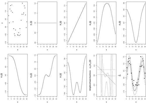
Figure 2. An example of a thin plate regression spline basis for the model yt = βt + εt. The basis functions for the smooth curve βt of a thin plate regression spline basis are shown. The first panel represents the data through which the smooth curve will be fitted. The next two panels represent the first two basis functions, which are defined as R1(t) = 1 and R2(t) = t. The other five basis functions (R3(t)–R7(t)) are thin plate spline-specific basis functions. Just as in standard regression, all basis functions Ri(t) are weighed by multiplying them with their corresponding αi coefficients. These weighted basis functions are then summed up, resulting in the smooth curve (with CI) in the last panel at the bottom right where the black dots again represent the data.

Figure 2. An example of a thin plate regression spline basis for the model yt = βt + εt. The basis functions for the smooth curve βt of a thin plate regression spline basis are shown. The first panel represents the data through which the smooth curve will be fitted. The next two panels represent the first two basis functions, which are defined as R1(t) = 1 and R2(t) = t. The other five basis functions (R3(t)–R7(t)) are thin plate spline-specific basis functions. Just as in standard regression, all basis functions Ri(t) are weighed by multiplying them with their corresponding αi coefficients. These weighted basis functions are then summed up, resulting in the smooth curve (with CI) in the last panel at the bottom right where the black dots again represent the data.

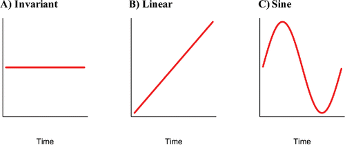
Figure 3. The three data-generating functions.

Figure 3. The three data-generating functions.

Figure 4. Average MSE values for both the TV-VAR (with 5, 10, and 20 basis functions) and the VAR model. The data were generated by the VAR model. A lower MSE value entails a better recovery of the true coefficient values. The number next to the β indicates its value.
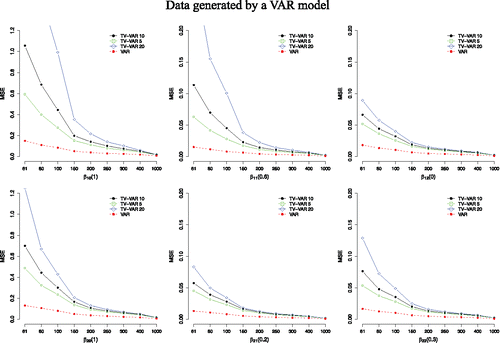
Figure 4. Average MSE values for both the TV-VAR (with 5, 10, and 20 basis functions) and the VAR model. The data were generated by the VAR model. A lower MSE value entails a better recovery of the true coefficient values. The number next to the β indicates its value.

Figure 5. Average coverage probabilities (CP) in % for both the TV-VAR (with 5, 10, and 20 basis functions) and the VAR model. The data were generated by the VAR model. A higher value entails capturing the true coefficient values better. The number next to the β indicates its value. CIs for both models were 95%.
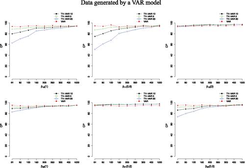
Figure 5. Average coverage probabilities (CP) in % for both the TV-VAR (with 5, 10, and 20 basis functions) and the VAR model. The data were generated by the VAR model. A higher value entails capturing the true coefficient values better. The number next to the β indicates its value. CIs for both models were 95%.

Figure 6. Average MSE values for both the TV-VAR (with 5, 10, and 20 basis functions) and the VAR model. The data were generated by the TV-VAR model. A lower MSE value entails a better recovery of the true coefficient values. The number next to the β indicates the maximum absolute value of β and the symbols describe how β changed over time.
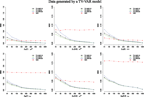
Figure 6. Average MSE values for both the TV-VAR (with 5, 10, and 20 basis functions) and the VAR model. The data were generated by the TV-VAR model. A lower MSE value entails a better recovery of the true coefficient values. The number next to the β indicates the maximum absolute value of β and the symbols describe how β changed over time.

Figure 7. Average coverage probabilities (CP) in % for both the TV-VAR (with 5, 10, and 20 basis functions) and the VAR model. The data were generated by the TV-VAR model. A higher value entails capturing the true coefficient values better. The number next to the β indicates the maximum absolute value of β and the symbols describe how β changed over time. CIs for both models were 95%.
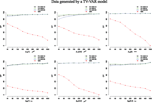
Figure 7. Average coverage probabilities (CP) in % for both the TV-VAR (with 5, 10, and 20 basis functions) and the VAR model. The data were generated by the TV-VAR model. A higher value entails capturing the true coefficient values better. The number next to the β indicates the maximum absolute value of β and the symbols describe how β changed over time. CIs for both models were 95%.

Figure 8. Daily positive affect (PA) scores for a male and a female involved in a romantic relationship.
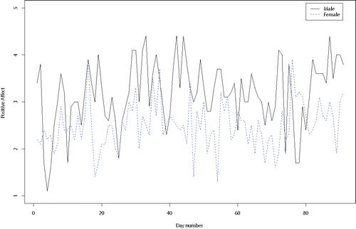
Figure 8. Daily positive affect (PA) scores for a male and a female involved in a romantic relationship.

Table 1. The eight different models to select from for male and female positive affect.

Table 2. Time-varying VAR model selection for PA of the male. Lowest fit indices are made bold.

Figure 9. Fitted values versus innovations of positive affect (PA) for both male and female. The innovations were homogenous and normally distributed.
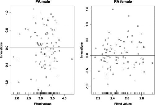
Figure 9. Fitted values versus innovations of positive affect (PA) for both male and female. The innovations were homogenous and normally distributed.

Figure 10. This figure shows the parameters of model 1 (Equation (Equation11)) for positive affect (PA) of the male and female. In model 1 all parameters were allowed to vary over time as smooth functions. The upper panel indicates, from left to right: (1) the intercept function, (2) the autoregressive function (or inertia) of PA of the male, and (3) the cross-lagged function (the effect of PA of the female on PA of the male). The lower panel has the same structure, but represents PA of the female, which could not be significantly predicted by her own PA nor the PA of her partner. Note that model 3 would result in the same figure, except for β11, t and β21, t, which in model 3 are constants of 0.25 and 0.06, respectively.
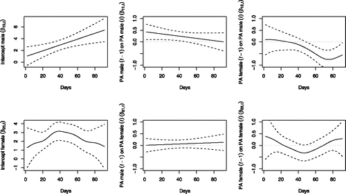
Figure 10. This figure shows the parameters of model 1 (Equation (Equation11(11) )) for positive affect (PA) of the male and female. In model 1 all parameters were allowed to vary over time as smooth functions. The upper panel indicates, from left to right: (1) the intercept function, (2) the autoregressive function (or inertia) of PA of the male, and (3) the cross-lagged function (the effect of PA of the female on PA of the male). The lower panel has the same structure, but represents PA of the female, which could not be significantly predicted by her own PA nor the PA of her partner. Note that model 3 would result in the same figure, except for β11, t and β21, t, which in model 3 are constants of 0.25 and 0.06, respectively.

Figure 11. Conceptual representation of the VAR model for positive affect (PA) of the male and the female. In the VAR model the dynamics are not allowed to change over time.
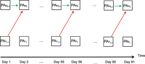
Figure 11. Conceptual representation of the VAR model for positive affect (PA) of the male and the female. In the VAR model the dynamics are not allowed to change over time.

Figure 12. Conceptual representation of the TV-VAR model for positive affect (PA) of the male and the female. In the TV-VAR model, the dynamics are allowed to change over time. In this dyad, the dynamics did indeed change. There was initially no effect of the female’s PA on the male’s PA, but this cross-lagged effect appeared halfway through the study (see the thin red arrow) and got stronger over time (see the thick red arrow).
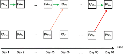
Figure 12. Conceptual representation of the TV-VAR model for positive affect (PA) of the male and the female. In the TV-VAR model, the dynamics are allowed to change over time. In this dyad, the dynamics did indeed change. There was initially no effect of the female’s PA on the male’s PA, but this cross-lagged effect appeared halfway through the study (see the thin red arrow) and got stronger over time (see the thick red arrow).