Figures & data
Figure 1. Graphical representation of the thought experiment. The left upper and lower panel show the data-generating network models containing five nodes, with, in the upper panel 10 edges, i.e., a fully connected network, or, in the lower panel, zero edges, i.e., an empty network. We refer to these two networks as the true data-generating networks. For both true underlying network structures, three network structures were randomly generated, yielding a sensitivity of 50% and a specificity of 90%. For simplicity, edge weights are of equal strength. Solely based on a visual comparison of the three randomly generated network structures, not knowing the true underlying network, one may be tempted to conclude that these three networks are very different, i.e., there is a great amount of heterogeneity present. In fact, all of this perceived “heterogeneity” is caused by sampling variation. (a) Fully connected case and (b) Empty case.
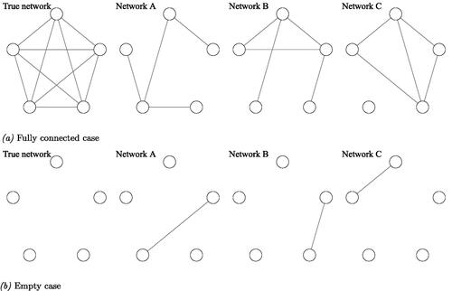
Figure 2. Contemporaneous and temporal data generating network models for each individual. The upper panel shows the synthetic-data network with eight nodes simulated to be a chain graph, i.e., 1–2, 2–3, etc. The middle panel shows the case-data network containing seven nodes estimated from clinical data of one subject measured over time. The lower panel shows the Geschwind-data network containing six nodes, estimated from clinical data of multiple subjects. The average contemporaneous and temporal networks are taken as the data-generating network structure for each individual in this study. Edges across networks are scaled to a maximum of 0.69, therewith edges between networks can be visually compared to one another. (a) Synthetic-data network, (b) Case-data network, and (c) Geschwind-data network.
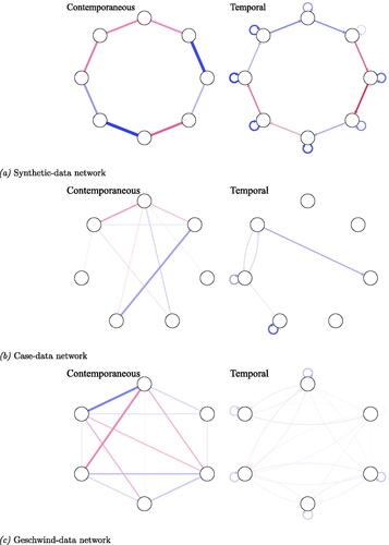
Figure 3. Output from graphical VAR. Three randomly selected individual networks estimated using the graphical VAR method, generated under the same synthetic-data network structure (for a visualization of the synthetic-data network see panel (b)) for two different time points (t = 50 and t = 400). Panel (a) shows the three individual contemporaneous networks when t = 50, panel (b) for t = 400, panel (c) shows their corresponding temporal networks when t = 50, and panel (d) for t = 400. (a) Contemporaneous networks for individual 1, 2, and 3 when t = 50, (b) Contemporaneous networks for individual 1, 2, and 3 when t = 400, (c) Temporal networks for individual 1, 2, and 3 when t = 50, and (d) Temporal networks for individual 1, 2, and. 3 when t = 400.
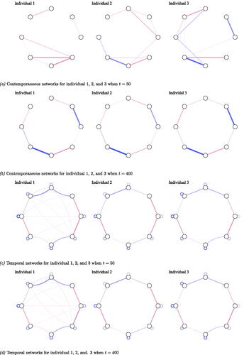
Figure 4. Correlations between node strength centrality calculated from individual networks estimated with graphical VAR. For the contemporaneous network, the correlation between strength centrality is depicted. For temporal networks, the correlations for two strength measures were computed: in-strength and out-strength. Correlations between strength measures of contemporaneous networks are highest for networks estimated under the Geschwind-data structure, while the in- and out-strength correlations are highest for networks generated under the synthetic-data structure.
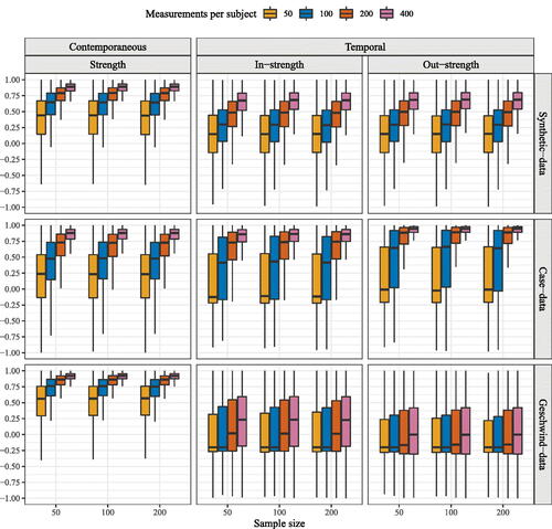
Figure 5. Density distribution of standardized edge weights for standard deviations of random effects for the multilevel VAR model. The vertical black dotted line represents the recommended cutoff of one standard deviation. Edges above or below these cutoff’s are seen as truly heterogeneous.
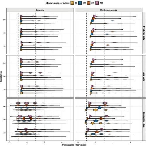
Figure 6. Percentage of homogeneous edges as estimated through GIMME for the synthetic-data, case-data, and Geschwind-data network structures.
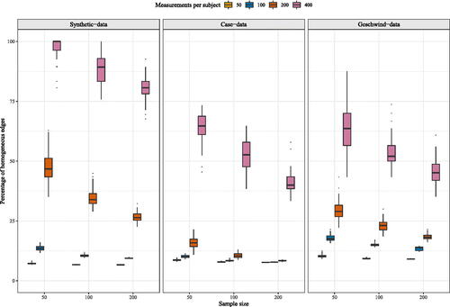
Figure A1. Output from graphical VAR. Three individual networks (contemporaneous and temporal) were generated under the same case-data network structure. Panel (a) shows the contemporaneous networks for t = 50, (b) for t = 400, (c) their corresponding temporal networks with t = 50, and (d) for t = 400. (a) Contemporaneous network for individual 1, 2, and 3 when t = 50, (b) Contemporaneous network for individual 1, 2, and 3 when t = 400, (c) Temporal network for individual 1, 2, and 3 when t = 50, and (d) Temporal network for individual 1, 2, and 3 when t = 400.
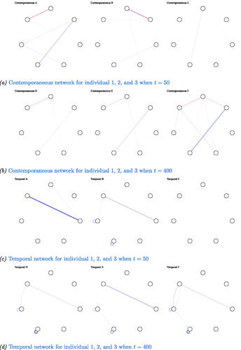
Figure A2. Output from Graphical VAR. Three individual networks (contemporaneous and temporal) were generated under the same Geschwind-data network structure. Panel (a) shows the contemporaneous networks for t = 50, (b) for t = 400, (c) their corresponding temporal networks with t = 50, and (d) for t = 400. (a) Contemporaneous network for individual 1, 2, and 3 when t = 50, (b) Contemporaneous network for individual 1, 2, and 3 when t = 400, (c) Temporal network for individual 1, 2, and 3 when t = 50, and (d) Temporal network for individual 1, 2, and 3 when t = 400.
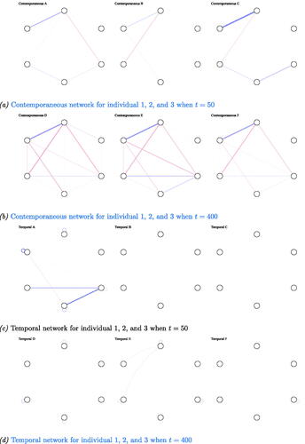
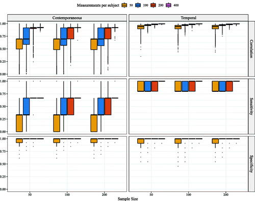
Figure B1. Sensitivity results for graphical VAR. Correlation, sensitivity, and specificity for contemporaneous and temporal individual networks for synthetic-data, case-data, and Geschwind-data network structures.
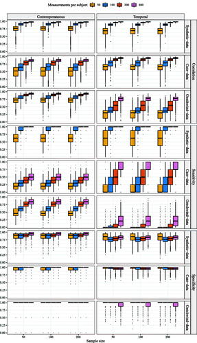
Figure C1. Sensitivity results for multilevel VAR. Correlation, sensitivity, and specificity are depicted for contemporaneous and temporal individual networks for synthetic-data, case-data, and Geschwind-data network structures. In line with previous simulation study results, sensitivity is 100% and specificity 0% as a result of all edges being estimated (see Epskamp et al. (Citation2018a). Therewith, the correlation between the data generating network model and the estimated network model is a better indication of the power of the estimation technique.
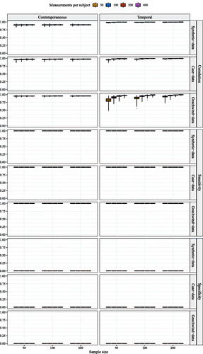
Figure D1. Sensitivity results for GIMME. Correlation, sensitivity, and specificity are depicted for contemporaneous and temporal individual networks as simulated under a structural VAR network and estimated using GIMME. More details on the simulation procedure and parameter values of the data generating network structure can be found in supplement B. Important to note here is that the diagonal of the temporal matrix is taken into account when computing the sensitivity to make the comparison between sensitivity results for GIMME, graphicalVAR, and mlVAR more straightforward.