Figures & data
Table 1. Reads sequenced and mapped for Epichloë-infected grasses genotyped by GBS.
Figure 1. Geographic distribution of genetic clusters of 206 E. uncinata isolates. Colors reflect the clusters assigned by the Bayesian information criterion. Individuals were clearly assigned to one of the three clusters, and only a few individuals showed a low signal of admixture. Individual-based principal component analysis was obtained from 6654 genotyped SNPs. The first principal component axis (PC1) accounts for most of the intrapopulation variety (15.6%), the second principal component axis (PC2; 6.5%) allows a good separation of three clusters, named Eu_P1 (aquamarine), Eu_P2 (orange), and Eu_P3 (purple), and the third principal component axis (PC3; 2%) allows good isolation of Eu_P3 from the other clusters.
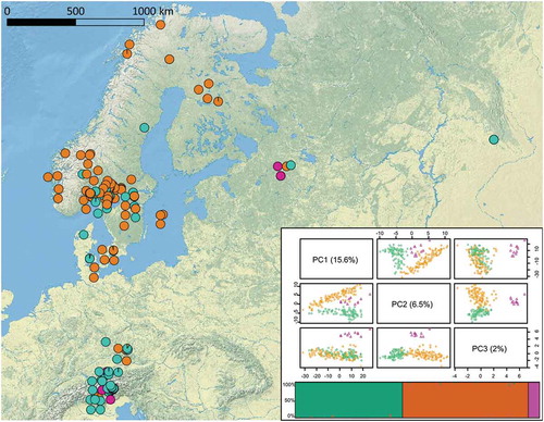
Figure 2. Geographic distribution of genetic clusters of 206 S. pratensis samples. Colors reflect the clusters found by the fastSTRUCTURE analysis. Individual-based principal component analysis obtained from 37 319 genotyped SNPs. Although the first principal component axis (PC1; 7.2%) does not allow a good discrimination of groups, plotting isolates using the second (PC2; 4.1%) and the third (PC3; 2.4%) axes groups them into three clusters, named Sp_P1 (red), Sp_P2 (yellow), and Sp_P3 (green).
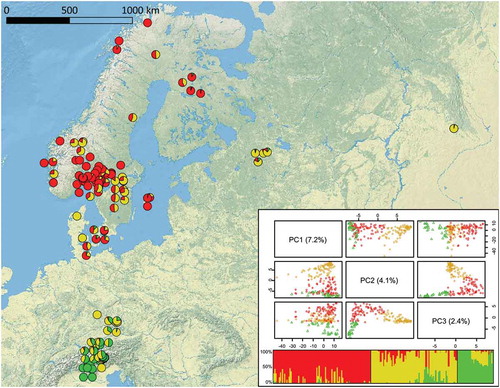
Figure 3. Geographic distribution of E. uncinata clusters. A. Eu_P1. B. Eu_P2. Pie charts show the level of admixture of the hosts according to the same colors shown in FIG. 2.
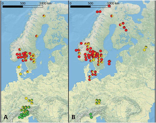
Table 2. Occurrence of endophyte strains in each S. pratensis subpopulation and total number of samples assigned to each subpopulation.
Figure 4. Tanglegram of the maximum likelihood phylogenies of Epichloë endophytes and their grass hosts. Trees were obtained with the software MEGA X and edited with FigTree. Labels were connected using the function tanglegram from the package dendextend. Straight lines, showing endophyte and host grass matches in the phylogenies, connect S. arundinaceum and L. perenne individuals to their respective endophytes, i.e., E. coenophiala, E. festucae, and E. siegelii, which were infecting an elite perennial ryegrass cultivar. E. uncinata strains and S. pratensis subpopulations are marked with the same colors used in FIG. 1 and FIG. 2, respectively.
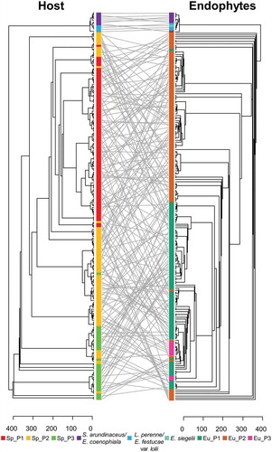
Figure 5. Variation of loline alkaloids in the three subpopulations of E. uncinata. The box plots are provided with pairwise comparisons between subpopulations using the Wilcoxon rank-sum test adjusted with the Bonferroni correction for multiple testing.
Figure 6. Plots on the left show the amount of NAL, NANL, and NFL in E+ S. pratensis as a function of total lolines: NFL is the main compound responsible for increasing levels of lolines. Plots on the right side show the relative percentage of each compound. In Eu_P2, at increasing levels of total lolines, the percentage of NANL increases, whereas the percentage of NAL decreases. Points lying on the same vertical line belong to the same sample. *Probability value of Kendall’s rank correlation test <10−4.

Figure 7. A, B. Scatterplots showing the correlations between the total amount of lolines and the percentage of reads mapped to the endophyte reference (A) but not to the plant reference (B). C, D. Scatterplots showing the correlations between the mycelial biomass and the total amount of lolines (C) and the percentage of reads mapped to the endophyte reference (D). The 95% confidence intervals (CIs) are shaded in gray. Kendall’s rank correlation coefficient (τ) values and respective P-values are shown.
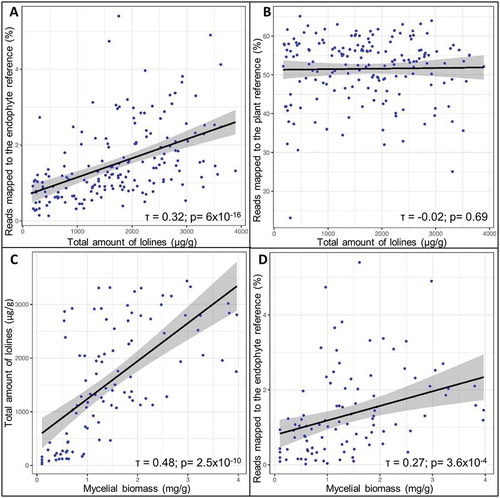
Figure 8. Variation in biomass in the three subpopulations of E. uncinata and S. pratensis. The box plots are provided with pairwise comparisons between subpopulations using the Wilcoxon rank-sum test adjusted with the Bonferroni correction for multiple testing.