Figures & data
Figure 1. Basic structure of a dynamic partially stratified estuary, showing: water column structure for velocity (showing both instantaneous–in this case ebb = u(z) and mean ‘estuarine circulation’ = u dotted) and density ρ with benthic and surface boundary-layers with and intermediate stratified later. The boundaries and internal shear produce turbulence which is dissipated at rate ε (the dotted line is an indicative law of the wall decay). The instantaneous velocity profile oscillates back and forth with the tidal ebb and flood generating a highly variable dissipation rate structure.
Table 1. Tidal channel bulk parameters as estimated from various studies.
Figure 2. Map showing A, New Zealand; B, Pelorus Sound and its main channel (blue), the Pelorus River, the large inlet of Keneperu Sound and the adjacent but unconnected Queen Charlotte Sound. C, Shows the study site Hikapu Reach, where the grey lines are 10 m contours. The square is the RDCP/Vector mooring and the diamond is the approximate location of the profiling vessel although this would move on its mooring.
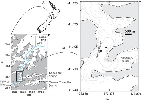
Figure 3. Section of Pelorus River flow rate as gauged at Bryants Crossing (41°18′S; 173°34′E). The horizontal bar shows the time of sampling.
Figure 4. Example Vector power spectral density (PSD) distribution showing a spectrum which met the acceptance criteria (black) and a rejected spectrum which did not (grey). Mooring vibration modes are identified with arrows. The two vertical lines show the frequency range over which the f−5/3 (grey solid sloping line) energy distribution is estimated. The dotted lines are the best-fit slope for the selected spectra.
Figure 5. A 2-day section of the RDCP velocity data showing A, depth at the mooring and the north-south current component at mid-depth (northward is ebb, positive and shaded), B, the north-south velocity distribution (m s−1) as a function of height above bed and C, velocity shear (s−1). The Vector is located at height 17 m.
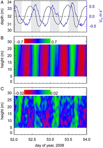
Figure 6. Tidal-cycle temporal averages of tidal principal axis along-channel (quasi-north-south) velocity profile from the RDCP. Hatched sections are outside the RDCP sample volume. The data were divided into 12.4 hour sections and time-averaged. The solid black line is the overall average (to the nearest 12.4 hours) and the shaded zone is the total average +/− the standard deviation at each depth. The dash-dot line is the cross-channel equivalent (arranged so that positive is westward so as to correspond to ebb). The averages were conducted over exact semidiurnal tidal periods. The scale of the inset box (showing north-south vs east west flow samples) is +/− 1 ms−1 in both axes.
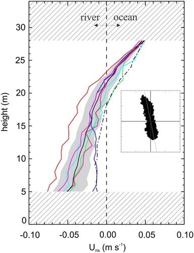
Figure 7. Example CTD profile showing A, temperature and salinity; B, density (sigma t = density – 1000 at atmospheric pressure); and C, buoyancy frequency squared.
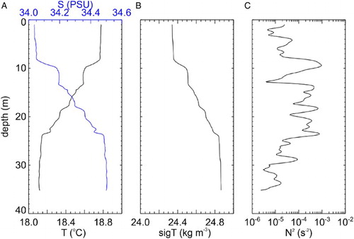
Figure 8. Velocimeter data showing A, total pitch and roll and velocity estimate correlation as a percentage (corr pcnt); and B, absolute velocity (the grey line is the equivalent depth bin of the RDCP). The εv estimate fitting parameters are shown in C, as slope marked as circles (shaded area as threshold) and the least squares fit (LSF) residual (line, with dashed line as threshold). Good fits are solid circles. Panel D, shows velocimeter depth pressure along with all the εv estimates. Good fits are solid circles.
Figure 9. Velocimeter estimates of εv A, as function of north-south velocity (measured values as open squares and solid squares are binned values with 0.1 m s−1 bins, error-bars shows + 1 standard deviation) so that positive u is the ebb tide (Northward flowing); and B, as function of tidal speed phase (radian) where 0-π is the flood, and π−2π is the ebb. The inset shows the phase construction.
Figure 10. A, Density profiles from the CTD offset by 0.5 kg m−3 (scale bar top right) captured at times marked by dashed lines connecting the two panels. The dashed lines show the respective 24.5 kg m−3 value. B, Energy dissipation rate εs (m2 s−3) from the shear SMS profiles along with the pressure at the velocimeter showing tidal height variation, and the shaded band is between two isopycnals (24.5 and 24.6 kg m−3) estimated from the VMP’s temperature and conductivity sensors (not the CTD, so the shaded band in panel B doesn’t exactly match the CTD in panel A).
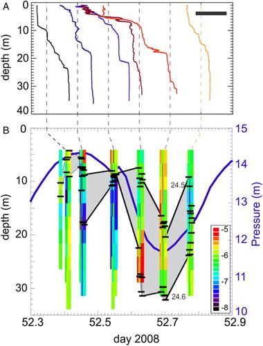
Figure 11. A, depth of velocimeter (add 17 m for full water depth) and depth-averaged northward-southward (northward = ebb) current from the RDCP. B, Offset density profiles as per A where the scale bar is 0.5 kg m−3 and with Rigr superimposed (plotted in inverse form log10[1/(4Rigr)] so that Rigr = 0.25 is 0, and reduced stability is greater in value, i.e. bright spots = ‘mixing’). The profiles are alternately solid and dashed to aid in identification.
![Figure 11. A, depth of velocimeter (add 17 m for full water depth) and depth-averaged northward-southward (northward = ebb) current from the RDCP. B, Offset density profiles as per Figure 10A where the scale bar is 0.5 kg m−3 and with Rigr superimposed (plotted in inverse form log10[1/(4Rigr)] so that Rigr = 0.25 is 0, and reduced stability is greater in value, i.e. bright spots = ‘mixing’). The profiles are alternately solid and dashed to aid in identification.](/cms/asset/19476982-2194-465d-81cb-c3436006db14/tnzm_a_1171243_f0011_c.jpg)
Figure 12. Comparison of dissipation rate estimates from velocimeter (εv) and shear microstructure (εs). Individual realisations of microstructure εs from the velocimeter depth are circles and the binned averages are the squares. The dashed line is the one-to-one fit. Fit A is through all the binned means and line B is excluding the shaded outlier as discussed in the text.
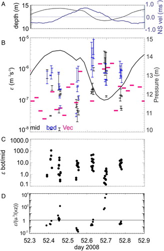
Figure 13. A, Depth of velocimeter (add 17 m for full water depth) and depth-averaged northward-southward (northward = ebb) current from the RDCP. B, Dissipation rate (ϵ) where the velocimeter estimates are pink horizontal lines extending over the duration of the data burst. The shear SMS estimates are shown as vertical lines bracketing the two shear probe estimates (black at depth of Vector velocimeter, blue at deepest point in profile). The velocimeter pressure is retained for reference. C, Ratio of SMS dissipation rates from deepest to velocimeter-depth bins. D, Average of ratio of εs to law of the wall dissipation for deeper half of water column.