Riparian management affects instream habitat condition in a dairy stream catchment

Figures & data

Figure 1. The Waikakahi Stream catchment (South Canterbury, New Zealand) showing the locations of the eight surveyed 1 km stream segments. The stream flows from west to east before it joins the Waitaki River c. 4 km upstream of the coast. All tributaries and the mainstem 1 km upstream of Site 8 are ephemeral.

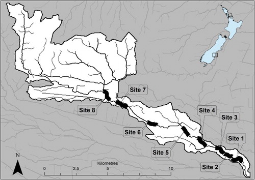
Table 1. Mean percentage values (and standard deviations) for instream habitat variables, including mesohabitat type, depths and sediment cover, for all 20 m sub-reaches combined (n = 115). Stream bed sediment categories were only for the visible areas of the stream bed (i.e. areas not obscured by deep water or aquatic macrophytes).

Mesohabitat types	Pool	Riffle	Slow run	Medium run	Fast run	Backwater
	2.7 (14.6)	4 (13.9)	48 (47.2)	14 (34)	31 (42.4)	0.4 (2.7)
Depths (m)	0–0.3	0.3–0.5	0.5–1.0	>1
	29.3 (36.2)	40.5 (33.9)	24.7 (27)	5.9 (15.1)
Stream bed sediment cover	Clay/mud/silt/sand	Fine gravel	Coarse gravel	Small cobble	Large cobble
	19.3 (29.5)	19.3 (19.8)	38.6 (28.4)	19.4 (21.6)	3.7 (8.1)
Fish cover types	Ub 0–0.3m	Ub 0.3–0.5m	Ov 0–0.3m	Ov 0.3–0.5m	Ov 0.5–1m	Ov >1m	Lwd m^2	Sb m^2	Mm m^2
	9.1 (20.2)	5.6 (16.5)	30.9 (38.8)	25.4 (37.5)	3.9 (15.8)	4.6 (17.3)	0.2 (1.1)	0.2 (3.2)	0.5 (0.3.2)

Ub, undercut bank; Ov, overhanging vegetation; Lwd, large woody debris; Sb, submerged branches; Mm, man-made cover.

Ub and Ov are the mean % linear cover of the 20 m sub-reach margins (i.e. 40 m in total over both banks). Lwd, Sb and Mm are the mean % stream bed cover of the wetted area of the 20 m sub-reaches.

Table 2. Mean percentages (and standard deviations) for the coverage of various riparian vegetation categories for all GDZ (n = 86).

Riparian category	Grazed pasture	Exotic grasses	Native and exotic grasses	Native and exotic grasses and shrubs	Native and exotic grasses, shrubs and trees	Swampy/emergent native and exotic grasses and herbs	Trees (without understorey vegetation)
	81.6 (12.5)	13.5 (12.3)	0.7 (2.11)	0.2 (1.0)	3.7 (6.82)	0.05 (0.5)	0.05 (0.5)

With the exception of wetland-type vegetation, the vegetation categories represent the successional stages from grazed pasture through to mature forest (a more detailed explanation of the vegetation category types can be found in Field protocol S1).

Table 3. Correlations from an exploratory regression analysis of all riparian and instream habitat variables.

Habitat variable	Riparian habitat variable
	Mean fenced area (m^2/GDZ)
	100 m	500 m	1000 m
Fine sediment (% cover)	—		↓
Bank slumping (m/reach)		—	—
Stock pugging (m/reach)	—	↓	↓
Overhanging veg. 0.5–1 m (% cover)	—	↑	↑
	Mean stock pugging (m/GDZ)
	100 m	500 m	1000 m
Fine sediment (% cover)		↑	↑
	Mean bank slumping (m/GDZ)
	100 m	500 m	1000 m
Undercut banks 0–0.3 m (% cover)		↑	↑
Depth 0–0.3 m (% of reach)	—	↑	—
Depth 0.5–1 m	—	↑	—
Mesohabitat diversity	—	—	↑
Stock pugging (m/reach)	—	—	↑
Undercut banks 0.3–0.5 m (% cover)		↓	↑
	Mean riparian veg. index score / GDZ
	100 m	500 m	1000 m
Mesohabitat diversity	—	↓	—
Undercut banks 0–0.3 m (% cover)	—	—	↑
Depth 0.3–0.5 m (% of reach)	—	↑	—
Depth >1 m (% of reach)	—	—	↓

Regressions were undertaken at three scales: 100 m reach scale n = 23; 500 m sub-segment scale n = 15; and 1000 m segment scale n = 8. Only results that were significant (P = <0.05) for regressions that relate to our hypotheses are shown. Moderate (R² = 0.3–0.5) and weak (R² < 0.3) significant positive relationships are denoted by vertical and upwards sloping arrows, respectively. Moderate (R² = 0.3–0.5) and weak (R² < 0.3) significant negative relationships are denoted by vertical (downwards pointing) and downwards sloping arrows, respectively. A horizontal dash denotes no significant relationship.

Figure 2. Regression between longitudinally weighted mean % fine sediment cover and mean fenced riparian area per 100 m of stream length (n = 23) for all GDZ within each stream segment (1000 m). Circle size represents the weight (0 through 10) applied to each % fine sediment response value according to the location of the 100 m reach within the 1 km survey segment. For example, fine sediment cover values from a reach at the top of a survey segments were weighed one 10th the value of a reaches at the bottom of the segment.

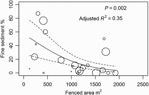
Figure 3. Summary of P, adjusted R² and sample size values for 10 individual (unweighted) sequential regressions of instream fine sediment cover vs mean fenced riparian area. The first regression, at the 100 m reach scale, compares sediment cover in instream survey reaches to fenced riparian area from adjacent GDZ. For each subsequent regression, the fenced riparian area is the mean from upstream GDZ incrementally included in the analysis.

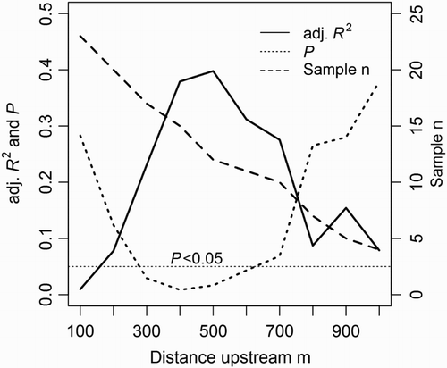
Figure 4. Mean deposited fine sediment cover from 100 m instream reaches regressed against the mean fenced riparian area of four upstream continuous 100 m GDZ (n = 15). The relationship shown (the fourth regression in a sequence of 10 regressions that included predictor variables from upstream areas in 100 m increments) had the strongest R² value.

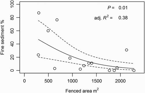
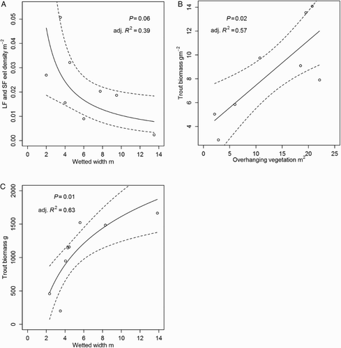
Figure 5. A, Linear regression between mean density (no./m²) of longfin and shortfin eels (combined) and wetted width (of instream survey reaches) in November 2012; B, mean trout biomass (g/m²) and overhanging (draping) vegetation expressed as mean % cover of the wetted width in November 2012; C, total trout biomass (g) and wetted width in March 2013.