Figures & data
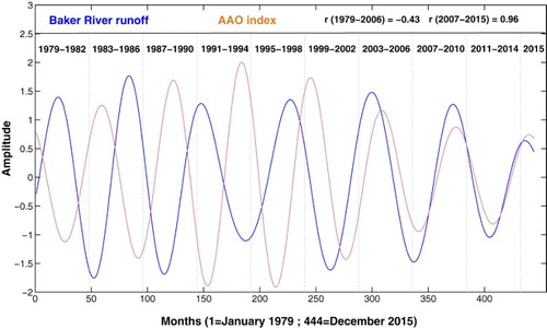
Figure 1. Baker River basin including the General Carrera and Bertrand lakes. The gauging station at Lake Bertrand is marked with a triangle (47°03′S; 72°48′W). Baker River and its largest tributaries, the Nef and Colonia rivers, are shown at the bottom of the map above the small village called Caleta Tortel. The Argentinian portion of General Carrera Lake is not shown on the map.
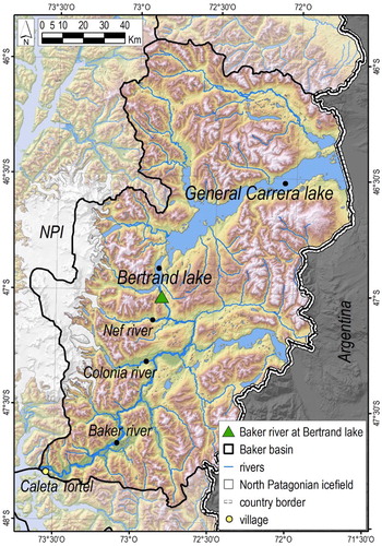
Figure 2. A, Baker River monthly runoff time series (Q, m3/s) from 1961 to 2015. Mean monthly runoff values were obtained from the Lake Bertrand sampling station (). Separations between decades are marked with vertical lines. B, Wavelet local power spectrum of runoff time series for the Baker River during the same time period. The red band associated with a periodicity of 12 months corresponds to the annual cycle. White lines indicate the cone of influence that delimits the region not influenced by edge effects. For A and B, the first and last observations correspond to January 1961 and December 2015, respectively. C, Wavelet global power spectrum. The grey line represents the α = 5% significance level. The annual cycle is clearly significant.
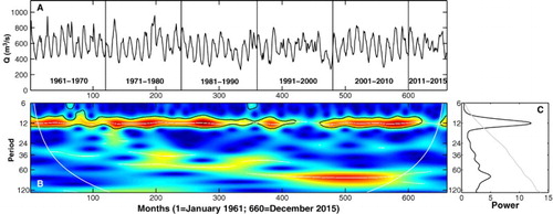
Figure 3. Root mean square fluctuation function F(s) on a logarithmic scale for the Baker River runoff time series between 1961 and 2015. Scaling range (between vertical lines) extends between 12 and 63 months (ca. 1 and 5.3 years), for which h(2) equals 0.94.
Figure 4. Determination coefficient (R2) calculated within rolling windows of length equal to 13. The first and second data points correspond to R2 values calculated between 1 and 13 months and between 2 and 14 months, respectively. The starting point of maximum and stable R2 values (above 0.95) was obtained for the rolling window marked with a vertical line at point 13, which corresponds to 12 months (1 year). The ending point of maximum R2 was obtained for the rolling window marked with a vertical line at point 43, which extends up to 63 months (5.25 years). According to these results, the scaling range extends between 1 and 5.25 years.
Figure 5. Hurst coefficients obtained for 1000 Monte Carlo simulated white noise time series and calculated with the DFA methodology. Lower and upper 95% confidence intervals are marked with vertical lines. The Hurst coefficient for Baker River runoff is marked with an arrow.
Figure 6. Generalised Hurst coefficients (h(q)s) estimated with the MF-DFA method obtained for 1000 Monte Carlo simulated white noise time series (triangles) and fractal Gaussian noise series with H = 0.94 (circles). h(q)s for the Baker River runoff time series are represented by squares connected by a continuous line. All time series have equal length (n = 660). Lower and upper 95% confidence intervals for white noise and fractional Gaussian noise time series are delimited by grey areas.
Figure 7. Reconstructed Baker River runoff and Antarctic Oscillation (AAO) Index time series using CWT. Scales between j1 = 62 and j2 = 64 months were used to reconstruct both series. Correlation coefficient (r) between Baker River runoff and AAO for (i) 1979–2006 period equals −0.43, and for (ii) 2007–2015 period equals 0.96.