Location and Activity Characterization of Gamma-Ray Point Sources Concealed in Shipping Containers Using Iterative Reconstruction and Modeling Cargo-Specific Attenuation

Figures & data

TABLE I RPM Descriptions and the Background Count Rates Added to the Simulated Measurements for Each Detector Type*

RPM Description	Scintillator Unit Size	Background (cps)
Two PVT scintillator panels stacked vertically either side of the traffic lane	60 $\times$ 203 $\times$ 3.8 cm PVT panel	5000
Four NaI scintillator crystals stacked vertically with alternating horizontal offset, either side of the traffice lane (see Fig. 1)	10.2 $\times$ 40.6 $\times$ 10.2 cm NaI crystal	2000 (100 at 662 keV)

*The background count rates represent conservative estimates for the types of detectors modeled in this work.^[16,17]

Fig. 1. Geometry defined in GEANT4 to simulate a shipping container passing through an RPM. All units are in centimeters. The dimensions of the cargo within the container are 587 $\times$ 235 $\times$ 233 cm, and the dimensions of the NaI detectors are 10.2 $\times$ 40.6 $\times$ 10.2 cm. The center, mid, and corner positions of the sources are depicted on the top- and side-view drawings.

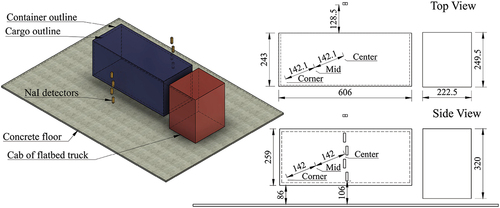
Fig. 2. Simulated counts measured by four PVT scintillator detectors in an RPM as a shipping container passes through with a 10-MBq 662-keV source at the container center, mid, or corner position. Error bars are estimated from the square root of the number of counts, assuming Poisson counting statistics. The detector positions are defined similarly to Fig. 1, with two PVT detectors on either side of the container as opposed to four NaI detectors, and the source in the corner position is closest to the left-side detectors.

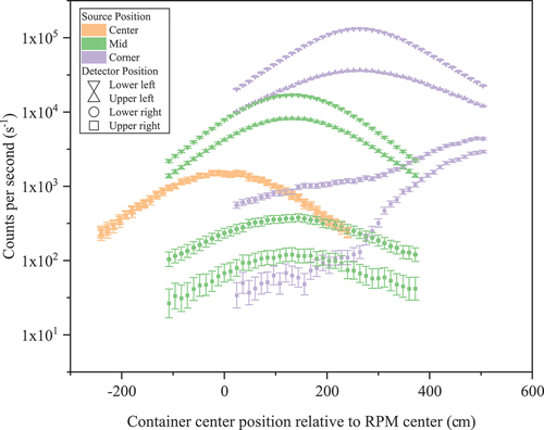
TABLE II Densities and Mass Attenuation Coefficients of Materials Used in This Work^[26]*

Material	Density (gcm^−3)	μg ($\times {10}^{-2}$) (cm^2g^−1)
Iron	7.874	7.346
NaI	3.667	7.395
PVT (C9H10)	1.032	8.356

*Mass attenuation coefficients are evaluated at 662 keV for each material.

Fig. 3. Values of $\mathrm{\ell }$ (arbitrary units) calculated from the optimum point-source solution in each voxel when a 3-MBq source is in the corner position, there is no cargo (0.0 gcm⁻³), and measurements are with the PVT-based RPM. $\mathrm{\ell }$ is shown at three cross sections through the voxelized shipping container, and the smallest $\mathrm{\ell }$ values indicate the most likely source positions. The green box is the outline of the container.

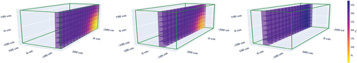
Fig. 4. Values of $\mathrm{\ell }$ (arbitrary units) calculated from the optimum point-source solution in each voxel when a 3-MBq source is in the center position, there is no cargo (0.0 gcm⁻³), and measurements are with the PVT-based RPM. $\mathrm{\ell }$ is shown at three cross sections through the voxelized shipping container, and the smallest $\mathrm{\ell }$ values indicate the most likely source positions. The green box is the outline of the container.

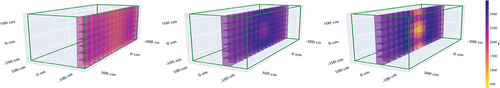
Fig. 5. Algorithm (a) activity, (b) localization, and (c) background estimation performance for a 10-MBq 662-keV source at the center, mid, or corner of a 20-ft shipping container. Results are after 30 iterations, and the true background count rates are 100, 2000, and 5000 for the NaI photopeak (NaI PP), NaI gross (NaI), and PVT data, respectively, as indicated by the solid horizontal lines in (c). The true source activity, 10 MBq, is indicated by the solid line in (a), and the size of one voxel is 40.5 $\times$ 36.3 $\times$ 36.1 cm.

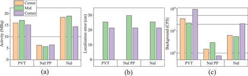
Fig. 6. Algorithm (a) activity, (b) localization, and (c) background estimation performance for a 10-MBq 662-keV source at the center, mid, or corner of a 20-ft shipping container containing a 0.2 gcm⁻³ iron cargo. Results are after 30 iterations, and the true background count rates are 100, 2000, and 5000 for the NaI photopeak (NaI PP), NaI gross (NaI), and PVT data, respectively, as indicated by the solid horizontal lines in (c). The true source activity, 10 MBq, is indicated by the solid lines in (a), and the size of one voxel is 40.5 $\times$ 36.3 $\times$ 36.1 cm.

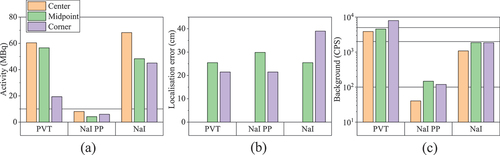
Fig. 7. Algorithm (a) activity, (b) localization, and (c) background estimation performance for a 10-MBq 662-keV source at the center, mid, or corner of a 20-ft shipping container containing a 0.6 gcm⁻³ iron cargo. Results are after 30 iterations, and the true background count rates are 100, 2000, and 5000 for the NaI photopeak (NaI PP), NaI gross (NaI), and PVT data, respectively, as indicated by the solid horizontal lines in (c). The true source activity, 10 MBq, is indicated by the solid lines in (a), and the size of one voxel is 40.5 $\times$ 36.3 $\times$ 36.1 cm.

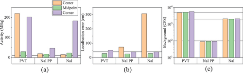
Fig. 8. Values of $\mathrm{\ell }$ (arbitrary units) calculated from the optimum point-source solution in each voxel when a 3-MBq source is in the mid position, there is a 0.2 gcm⁻³ iron cargo, and measurements are the gross counts with the NaI-based RPM. $\mathrm{\ell }$ is shown at three cross sections through the voxelized shipping container, and the smallest $\mathrm{\ell }$ values indicate the most likely source positions. The green and gray boxes are the outlines of the container and cargo, respectively.

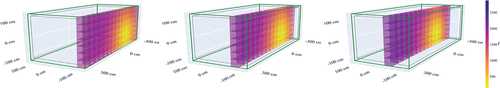
Fig. 9. Values of $\mathrm{\ell }$ (arbitrary units) calculated from the optimum point-source solution in each voxel when a 3-MBq source is in the mid position, there is a 0.2 gcm⁻³ iron cargo, and measurements are the photopeak counts with the NaI-based RPM. $\mathrm{\ell }$ is shown at three cross sections through the voxelized shipping container, and the smallest $\mathrm{\ell }$ values indicate the most likely source positions. The green and gray boxes are the outlines of the container and cargo, respectively.

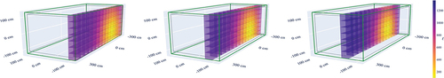
Fig. 10. Brute-force implementation of MLEM PS with μ_g values in the range 0.008 to 0.031 cm⁻¹. The results are for a PVT RPM with a 10-MBq source concealed in a 0.2 gcm⁻³ iron cargo, with the source in the center (left column), mid (middle column), and corner (right column). The likelihood of the optimum solution, the activity, and the localization error are shown. The black dashed line represents μ_g at the optimum solution, and the red dashed line is the true μ_g.

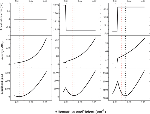
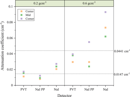
Fig. 11. Optimum attenuation factors determined using MLEM PS and a brute-force search over possible attenuation factors for the gross-count PVT and NaI data sets and the NaI photopeak data set (NaI PP). The horizontal dashed lines represent the true attenuation factors in the 0.2 gcm⁻³ and 0.6 gcm⁻³ cargo in units of cm⁻¹.

K. D. JARMAN et al., “Bayesian Radiation Source Localization,” Nucl. Technol., 175, 1, 326 (2011); https://doi.org/10.13182/NT10-72.

 Web of Science ®Google Scholar

E. A. MILLER et al., “Combining Radiography and Passive Measurements for Radiological Threat Localization in Cargo,” IEEE Trans. Nucl. Sci., 62, 5, 2234 (2015); https://doi.org/10.1109/TNS.2015.2474146.

 Web of Science ®Google Scholar

K. O. M. J. BERGER et al., “XCOM: Photon Cross Sections Database,” National Institute of Standards and Technology; https://www.physics.nist.gov/PhysRefData/Xcom/html/xcom1-t.html ( accessed Oct. 22, 2022).

 Google Scholar