Optimizing the Implementation of Small Modular Reactors into Ontario’s Future Energy Mix

Figures & data

TABLE I Endogenous Variables in CPLEX Model

TC	Total cost of model instance period ($/period)
K0, j	Preexisting capacity of j’th-type power plant within provincial energy mix when model instance initiates (kW)
GhgEmj	CO2 emissions for j’th-type power plant (gCO2/kW∙h)
CFj	Capacity factor for j’th-type power plant
knj	Newly installed capacity by model for j’th-type power plant (kW)
kj	Total installed capacity, preexisting and new, for j’th-type power plant (kW)
xi, j	Energy output during i’th time step for j’th-type power plant (kW∙h)
i	i ∈ {1, 2, 3, …, Years} Years: number of hours in a model instance (3 years = 26 280 h)
PlantTypej	PlantTypej ∈ {1: CANDU-based nuclear, 2: large hydropower, 3: small hydropower, 4: wind, 5: PV, 6: natural gas, 7: biomass/Other, 8: SMR-based nuclear}
a, b, c, d, e, f, g, h	Total energy output by each power plant (a = 1, … h = 8) during model instance (kW∙h)
j	j ∈ {1, 2, 3, …, N} N: Number of plant types in model instance
Accumj	Accumulating variable for j’th plant type, used to track iterations for later in postprocessing

TABLE II Exogenous Variables in CPLEX Model

FCRj	The annual fixed charge rate of the j’th power plant
Loadi	Demand on power grid during i’th time step (kW)
Fixedj	Sum of annual fixed costs for j’th-type power plant ($/kW∙yr)
Variablej	Sum of variable cost for j’th-type power plant ($/kW∙h)
CTn	Carbon tax for j’th-type power plant ($/kW∙h)
MaxCapj	Maximum installable capacity value based on remaining potential and preexisting capacities of j’th-type power plant (kW)
CapLimj	Available capacity limit (kW)
PVAvailabilityj	Hourly availability profile of PV potential, based on favorable yearly weather profile for Ontario
WindAvailabilityj	Hourly availability profile of wind potential, based on favorable yearly wind profile for Ontario
EmLim	Total annual CO2 emissions limit allowed by provincial regulations (g CO2/kW∙h)
MaxLoad	Maximum load demand in single hour across all time steps in model instance (kW)
CapRM	Capacity reserve margin, typically valued from 10% to 15% depending on demand throughout year
K0,1’, K0,1”, K0,1”’	Installed CANDU capacity variations
σ	Average expected transmission losses
ζ	Projected demand increase for model instance
Φmax,j, Φmin,j	Minimum and maximum output power levels, respectively, for j’th power plant
δI,j, δD,j	Maximum increase and decrease rate of changes of power outputs for j’th power plant, respectively
λ	Effective CANDU capacity reducing factor
Ωn	Milestone capacity values for application of NOAK cost reductions to SMR installed capacity
α	NOAK coefficient for cost reductions
n	Postprocessing counter, where n ∈ {1, 2, 3, 4}
Spring	Ranges of i corresponding to three spring seasons during model period: i ∈ {1896, …, 4086}, {10656 … 12846}, {19416 … 21606}
Fall	Ranges of i corresponding to three fall seasons during model period: i ∈ {6276 … 8466}, {15036 … 17226}, {23796 … 25986}

TABLE III Exogenous Variable Input Values for Various Power Plant Types

	Nuclear (CANDU)	Hydropower (Large)	Hydropower (Small)	Natural Gas	Biomass	SMR (GE Hitachi)	SMR (NuScale)
CPLEX Input Arrays	j = 1	j = 2	j = 3	j = 6	j = 7	j = 8	j = 8
Overnight capital cost ($/kW)	6276	6160	6930	1433	4650	3400	4000
Lifetime (yr)	30	30	30	20	30	60	60
Fixed O&M ($/kW∙yr^−1)	125.37	92	100	18.25	116	148.79	145
Annual fixed cost (¢/kW∙yr^−1)	33 457	29 733.33	33 100	8990	27 100	20 545.53	22 083.33
Variable O&M cost (¢/kW∙h)	0	0.33	1.67	0.28	0.18	0.10	0.095
Rate of output maximum increase (1/h)	0.60	0.05	0.05	0.44	0.31	0.60	0.60
Rate of output maximum decrease (1/h)	0.60	0.05	0.05	0.31	0.58	0.60	0.60
Fuel cost (¢/kW∙h)	1.45^a	0	0	2.44	2.16	1.10^a	1.10^a
Transmission costs (¢/kW∙h)	0	0.15	0.15	0	0.15	0	0
Total variable unit cost (¢/kW∙h)	1.45	0.48	1.82	2.72	2.49	1.20	1.20
Carbon tax (¢/kW∙h)	0	0	0	1.77	0	0	0
	Wind	PV
CPLEX Input Arrays	j = 4	j = 5
Overnight capital cost ($/kW)	2600	2140
Lifetime (yr)	20	20
Fixed O&M ($/kW∙yr^−1)	23	26
Annual fixed cost (¢/kW∙yr^−1)	15 300	13 300
Variable O&M cost (¢/kW∙h)	0	0
Fuel cost (¢/kW∙h)	0	0
Transmission costs (¢/kW∙h)	0.15	0.15
Total variable unit cost (¢/kW∙h)	0.15	0.15
Carbon tax (¢/kW∙h)	0	0

*References 2, 11, 14, 21, 29, and 32.

^aFuel cost includes 10 ¢/kW for future disposal.

Fig. 1. Projected demand curve for peak summer and winter demand over 20-year period from IESO’s 2021 annual planning outlook.^[6]

Fig. 2. CANDU reactor refurbishment and decommissioning schedule.^[6]

Fig. 3. Optimized 2055 energy mix with (a) GE Hitachi candidate SMR introduction and (b) NuScale iPWR candidate SMR introduction.

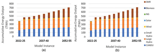
Fig. 4. Proportionate contributions to the average hourly load in the final model instance of the optimized scenario.

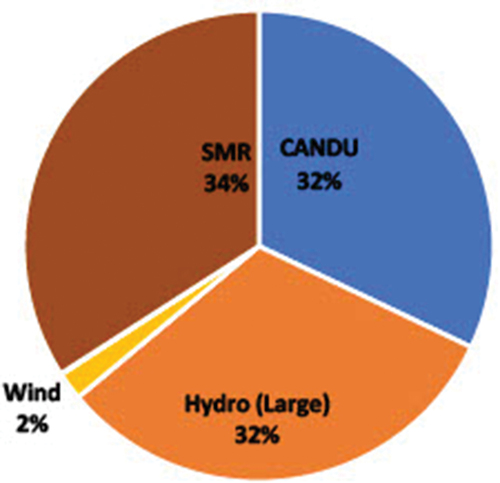
Fig. 5. IESO’s evaluation of Ontario’s energy adequacy given existing capabilities.^[6]

Fig. 6. Optimized 2055 installed capacities with (a) GE Hitachi candidate SMR introduction and (b) NuScale iPWR candidate SMR introduction.

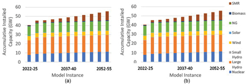
Fig. 7. Evaluation of energy adequacy of Ontario’s accumulative energy output in optimized GE Hitachi SMR scenario.

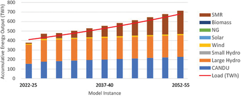
Fig. 8. Comparison of the growing average demand alongside the OBJ values for the GE Hitachi and no-SMR optimized scenarios. A trendline is included to compare the GE Hitachi OBJ values with a linear trend.

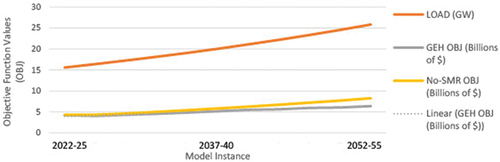
Fig. 9. Optimized 2055 no-SMR scenario: (a) installed capacity values and (b) accumulative energy output.

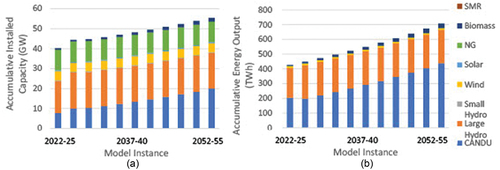
Fig. 10. Comparison of scenario OBJ values over time. The NuScale (NS) and GE Hitachi (GE) lines are too close to distinguish.

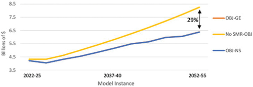
Fig. 11. Comparison of OBJ values of new GE Hitachi SMR scenario with no starting capacity (blue) and an initial investment of 2 GW into SMR capacity (orange). Agreeable results were found for a NuScale-based scenario.

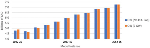
Fig. 12. Various projected learning curves corresponding to approximate costs at 0 GW installed (FOAK) and 10 to 16 GW installed (NOAK). For this case, existing CANDU capacity has been ignored.^{[4,5,33,36,37]}

Fig. 13. A comparison of the installed capacity values for SMRs versus CANDU reactors when (a) varying the total variable cost (fuel and variable O&M combined) and (b) varying the total fixed cost (OCC and fixed O&M combined).^{[4,5,33,36,37]}

Fig. 14. Projected accumulative energy output per model instance in constant CO₂ pricing scenario.

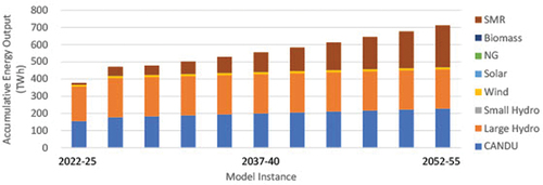
Fig. 15. Projected accumulative energy output per model instance in a scenario with no CO₂ pricing.

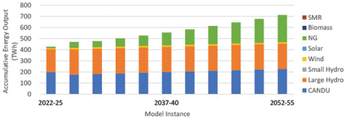
Fig. 16. Accumulative energy output from 2.5% annual increasing demand scenario. As expected, the resulting SMR output increased dramatically.

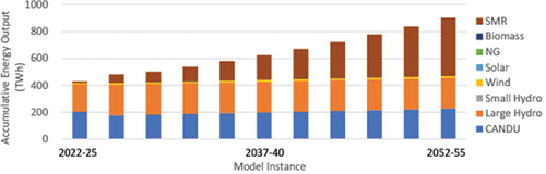
Fig. 17. Accumulative energy output from static load scenario. Without the increasing demand, it follows that SMR usage should be reduced overall, acting only to replace more expensive plant types.

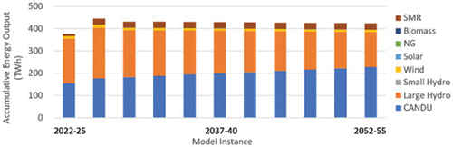
Fig. 18. Projected accumulative energy output from high SMR cost scenario (100% increase). With the significant increase in associated costs, SMRs are no longer effective in the economically optimized model.

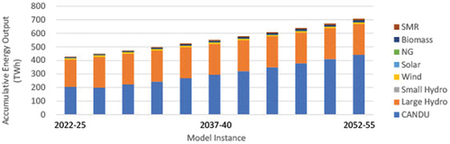
Fig. 19. Projected accumulative energy output from 50% SMR cost increase scenario. SMR usage has dropped significantly in lieu of CANDU use, though it is still viable to a small degree.

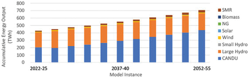
Fig. 20. Sensitivity analysis of the effect of varying fixed and variable SMR cost values on installed SMR capacity. Costs are represented as a fractional percentage of the original fixed and variable costs used in the optimized scenario, and the installed SMR capacity surpassed 1 GW at 177.6%, or a 77.6% increase from the original values.

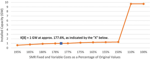
TABLE A.I Input Values for Model Constants

K0,1’	7778 MW	Installed CANDU capacity variations over time
K0,1”	8889 MW
K0,1”’	9172 MW
K0,1””	9989 MW
σ	0.04%	Average expected transmission losses
ζ	1.05%	Projected demand increase per model instance
${\phi }_{max,j},$${\phi }_{min,j}$	j = 1 0.95, 0.76	Minimum and maximum output power levels, respectively, for j’th power plant
	j = 2 1, 0
	j = 3 1, 0
	j = 4 1, 0^a
	j = 5 1, 0^a
	j = 6 1, 0
	j = 7 1, 0
	j = 8 1, 0.40
δI,j, δD,j	j = 1 0.60, 0.60	Maximum increase and decrease rate of changes of power outputs for j’th power plant, respectively
	j = 2 0.05, 0.05
	j = 3 0.05, 0.05
	j = 4 1, 0^a
	j = 5 1, 0^a
	j = 6 0.82, 0.75
	j = 7 0.31, 0.58
	j = 8 0.60, 0.60
λ	0.864	Effective CANDU capacity reducing factor
Ωn, n = 1	2 GW	Milestone capacity values for application of NOAK cost reductions to SMR installed capacity
Ωn, n = 2	4 GW
Ωn, n = 3	6 GW
Ωn, n = 4	8 GW
α	12%	NOAK coefficient for cost reductions

^aThe minimum/maximum values for j = 4, 5 (wind, PV) are determined by their availability profiles.

NUCLEAR POWER TECHNOLOGY DEVELOPMENT SECTION, “Status of Advanced Light Water Reactor Designs,” International Atomic Energy Agency (May 2004); https://www-pub.iaea.org/MTCD/Publications/PDF/te_1391_web.pdf (current as of May 20, 2022).

 Google Scholar

“2030 Emissions Reduction Plan: Clean Air, Strong Economy,” Government of Canada (July 12, 2022); https://www.canada.ca/en/services/environment/weather/climatechange/climate-plan/climate-plan-overview/emissions-reduction-2030.html (current as of May 20, 2022).

 Google Scholar

M. MCCLEARN, “Ontario Eyes Hydroelectric Projects as Demand for Power Rises,” The Globe and Mail (Jan. 23, 2022).

 Google Scholar

J. M. HOPWOOD, M. SOULARD, and R. LALONDE, “Advanced CANDU Reactor Design for Operability,” Proc. Int. Conf. Global Environment and Advanced Nuclear Power Plants (GENES4/ANP2003), Kyoto, Japan, September 15–19, 2003.

 Google Scholar

“Nuscale’s Affordable SMR Technology for All,” NuScale Power LLC (Mar. 2020); https://www.nuscalepower.com/newsletter/nucleus-spring-2020/featured-topic-cost-competitive (current as of May 20, 2021).

 Google Scholar

K.-H. MOON and S.-S. KIM, “An Exploratory Study on a Target Capital Cost and Cost Reduction Methodologies of Innovative SMR in Korea,” Transactions of the Korean Nuclear Society Virtual Spring Meeting, 2020.

 Google Scholar

“Ontario’s Supply Mix,” Independent Electricity System Operator (Oct. 2020); https://www.ieso.ca/en/Learn/Ontario-Supply-Mix/Ontario-Energy-Capacity (current as of May 5, 2020).

 Google Scholar

B. HEARD, “SMRs: Small Modular Reactors in the Australian Context,” Minerals Council of Australia (2021).

 Google Scholar

“Annual Planning Outlook, Ontario’s Electricity System Needs: 2023-2042,” Independent Electricity System Operator (2021).

 Google Scholar

B. WILSON, “Nuclear Feasibility for a New Zealand System,” Auckland University of Technology (2009).

 Google Scholar

“The Economics of Small Modular Reactors,” SMR Start (2017).

 Google Scholar

CANTEACH, “The Conventional Side of the Station,” CANDU Fundamentals, p. 261, Ontario Power Generation.

 Google Scholar