Presentation of the xM3 Test Case of the P2M Simulation Exercise and Modeling with the Fuel Performance Code ALCYONE

Figures & data

TABLE I Main Characteristics of the xM3 Rodlet

xM3 Segment
Rod length (mm)	522
Pellet stack length (mm)	441
Plenum length (mm)	44
Diametral gap (μm)	170
Rod pressure (He) (bar)	20
Fuel Pellet
Outer diameter (mm)	8.2
Height (mm)	10
Enrichment (wt% ^235U)	4.5
Grain size (μm)	30
Porosity (%)	4.7
Cladding
Outer diameter (mm)	9.5
Thickness (mm)	0.57

Fig. 1. Power histories and axial power profiles during the xM3 power ramp.

Fig. 2. Overview and details of the etched fuel cross section cut near the PPN after the xM3 power ramp.

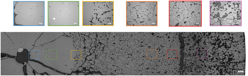
Fig. 3. Pore fractional area at selected pellet radii.^[9]

Fig. 4. Grain size determined at selected pellet radii according to the ASTM procedure.^[9]

Fig. 5. EPMA radial profiles of Cs and Xe after the xM3 power ramp.^[9]

Fig. 6. 1.5D scheme in the ALCYONE code (mesh is indicative).

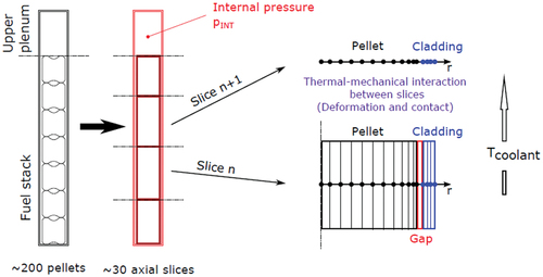
Fig. 7. U-O phase diagram calculated with the TAF-ID and OC (adapted from Introni et al.^[32]) compared to measurements of the solidus and liquidus temperatures (blue squares) by Manara et al.^[31] $x_O$ is the oxygen mole fraction of $\mathrm{U}{\mathrm{O}}_{2\pm \mathit{x}}$.

TABLE II Grouping of Fission Products and Actinides for the Thermodynamic Equilibrium Calculations with OC and the TAF-ID

He	U	Pu	O	Ba	Zr	Cs	I	Te	Mo	Ru	Pd	Ce	La	Gd
Xe	U	Pu	O	Ba	Zr	Cs	I	Te	Mo	Ru	Pd	Ce	La	Eu
Kr		Np		Sr	Nb	Rb	Br	Se		Tc	Sn	Pr	Y	Sm
He		Am						Ge		Rh	Sb			Gd
		Cm						As						Nd
														Pm

Fig. 8. Calculated liquid fuel fractions in irradiated UO₂ as a function of temperature and burnup.

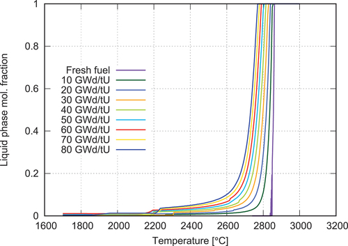
Fig. 9. Calculated evolution of the phase fractions with temperature in a fuel of average burnup 30 GWd/tU⁻¹: (a) all phases and (b) liquid phases.

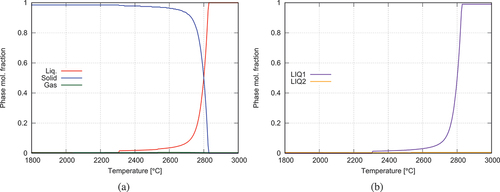
Fig. 10. Elemental composition of the immiscible liquid phases LIQ1 and LIQ2 as a function of temperature in a fuel of average burnup 30 GWd/tU⁻¹.

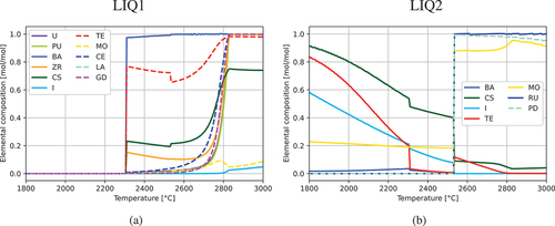
Fig. 11. Comparison of the calculated solid-liquid phase transition for a 30 GWd/tU⁻¹ fuel considering all phases and only the fluorite matrix.

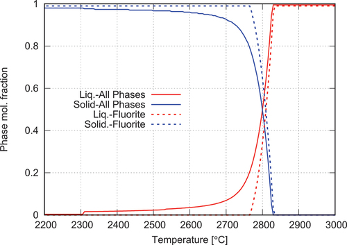
Fig. 12. TAF-ID estimates of the solidus $T_{\mathit{sol}}$ and liquidus $T_{\mathit{liq}}$ temperatures as a function of the fuel burnup compared to correlations from the open literature. $T_{\mathit{melt}}$ refers to the melting temperature when the solidus and liquidus temperatures are equal in the correlation.

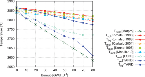
Fig. 13. Model implemented in ALCYONE for the liquid fuel fraction compared to the TAF-ID calculation results for a fuel of average burnup 30 GWd/tU⁻¹.

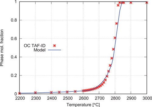
Fig. 14. Model implemented in ALCYONE for the heat capacity compared to the TAF-ID calculation results for a fuel of average burnup 30 GWd/tU⁻¹.

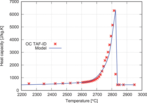
Fig. 15. Evolution of the thermal strain with temperature implemented in ALCYONE for a fuel of average burnup 30 GWd/tU⁻¹.

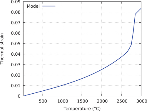
Fig. 16. Calculated and measured clad outer diameters before and after the xM3 power ramp.

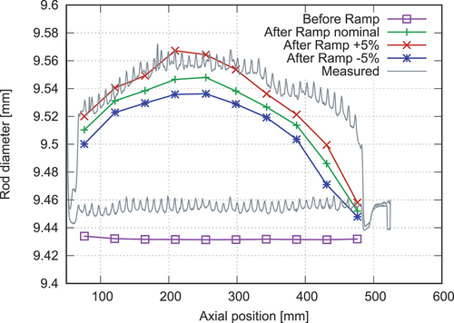
Fig. 17. Calculated and measured clad residual strains as a function of the local LHGR.

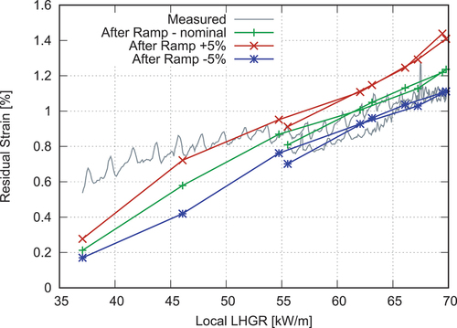
Fig. 18. Comparison of the calculated rod elongation with the experimental measurements performed during the xM3 power ramp.

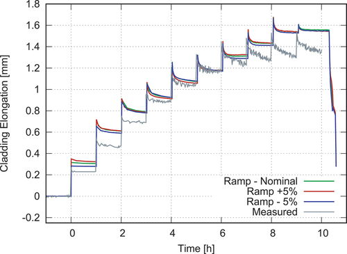
Fig. 19. Calculated radial profiles of temperature at RTL and PPN. The solidus and liquidus temperatures and the 1800°C isotherm are also indicated.

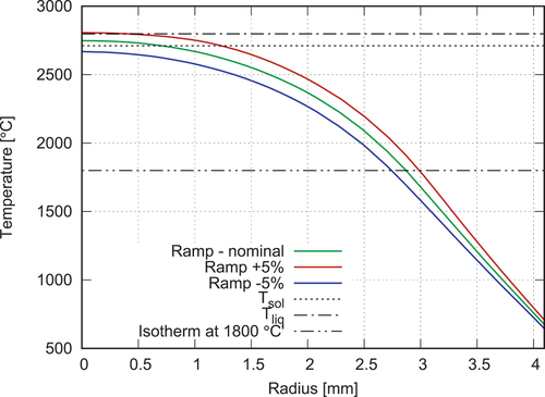
Fig. 20. Calculated radial profiles of the liquid fuel fraction at RTL and PPN.

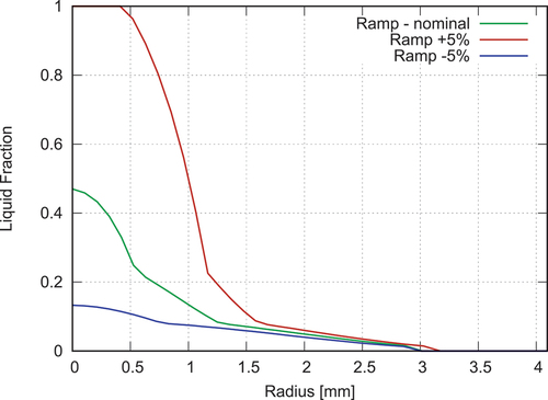
Fig. 21. Calculated axial profiles of the melting fuel radii at RTL, with the measured rod diameter after the power ramp (right y-scale). The radii of the inner porous and pore-free rings are also indicated.

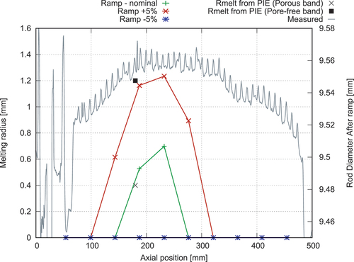
Fig. 22. (a) Calculated axial profiles of the pellet-clad gap at the end of the power ramp compared to the measured cold, residual, and relocated gaps. (b) Calculated axial profiles of the residual pellet diameter compared to the estimates by LOM.

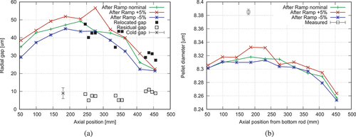
Fig. 23. Calculated radial profiles of Xe at RTL and at PPN. The measured EPMA profile is also indicated.

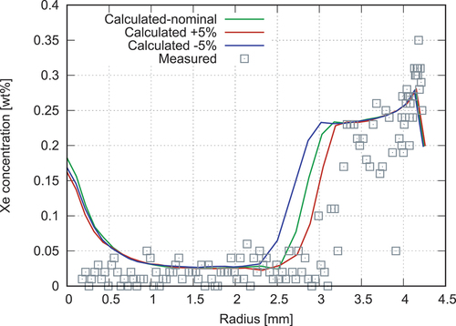
Fig. 24. Calculated FGR kinetics during the xM3 power ramp.

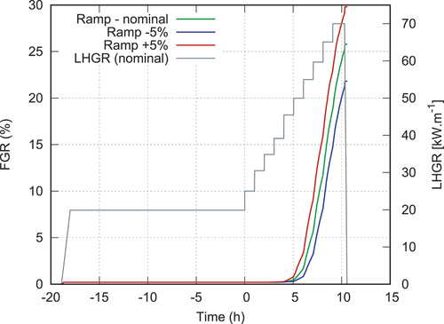
Fig. 25. Calculated radial profiles of porosity (initial porosity plus fission gas bubbles) at RTL and PPN compared to the measurements.

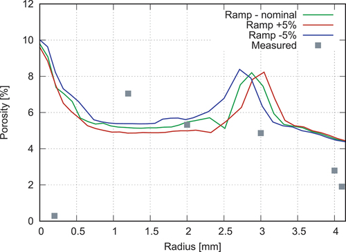
Fig. 26. Radial profile of porosity calculated at the end of the plateau at 70 kW/m considering a 4.7% initial porosity.

Fig. 27. Calculated evolution of the porosity at the pellet center and at PPN during the xM3 power ramp.

Fig. 28. Calculated evolution of the temperature at the pellet center during the xM3 power ramp with and without coupling with the pore migration mechanism.

Fig. A.1. (a) Setup for gap measurement and (b) recorded load displacement curves illustrating the principle of the measurement (reproduced from Ref. [9]).

H.-U. ZWICKY, “Post-Irradiation Examinations of Ramped Rodlets xM1, xM2 and xM3,” Studsvik Technical Report N-12/125 Rev. 1, STUDSVIK-SCIP-II-140, Studsvik (2012).

 Google Scholar

C. INTRONI et al., “Phase-Field Modeling with the TAF-ID of Incipient Melting and Oxygen Transport in Nuclear Fuel During Power Transients,” J. Nucl. Mater., 556, 153173 (2021); http://dx.doi.org/10.1016/j.jnucmat.2021.153173.

 Web of Science ®Google Scholar

D. MANARA et al., “Melting of Stoichiometric and Hyperstoichiometric Uranium Dioxide,” J. Nucl. Mater., 342, 1, 148 (2005); http://dx.doi.org/10.1016/j.jnucmat.2005.04.002.

 Web of Science ®Google Scholar