Direct Comparison of High-Order/Low-Order Transient Methods on the 2D-LRA Benchmark Problem

Figures & data

Fig. 1. 2D-LRA geometry.¹¹

Fig. 2. Example power evolution during the 2D-LRA transient on a 1 cm mesh.

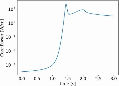
Fig. 3. Assembly power densities normalized to 1 W/cm³ at steady state, error with respect to results by Smith.¹²

TABLE I Sensitivity of the Transient Results on Time Step Size: Comparison with a Fine-Time Solution

	10^−5 s Solution	10^−4 s (Percent Relative Difference)	10^−3 s (Percent Relative Difference)
Time to first peak (s)	1.44545	0.04	0.45
Power at first peak (W/cm^3)	5448.7	0.03	0.43
Power at second peak (W/cm^3)	792.80	0.05	0.16
Power at t = 3 s (W/cm^3)	98.06	0.02	0.12

Fig. 4. Time stepping scheme for transient HOLO methods.

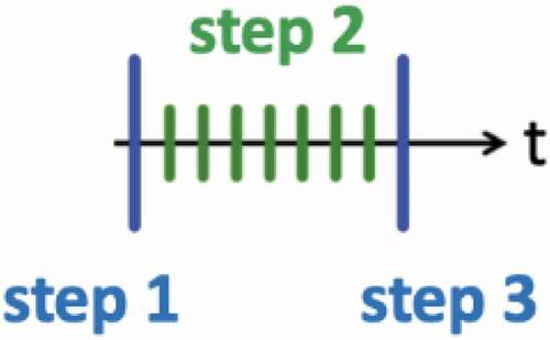
Fig. 5. Example reactivity evolution during the 2D-LRA transient on a 1 cm mesh.

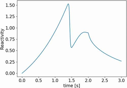
Fig. 6. Summary of HOLO methods and their relationships.

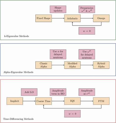
Fig. 7. Power profile shows that the fixed shape method is inadequate.

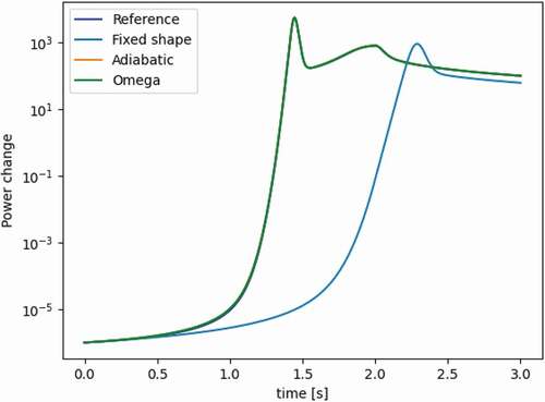
Fig. 8. Zoom-in to the first peak.

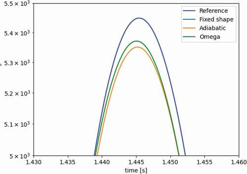
Fig. 9. Values of k-balance over time.

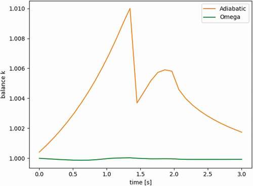
Fig. 10. Prompt frequencies as calculated by the omega method (in units of inverse seconds).

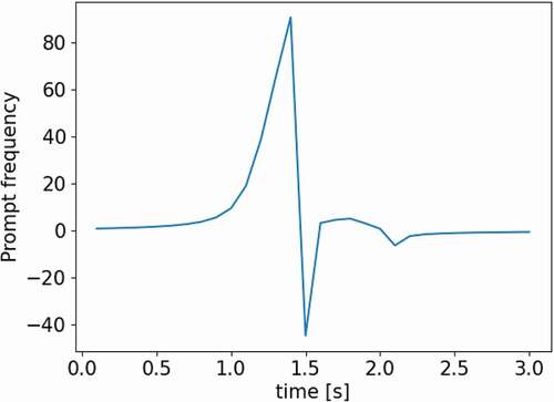
Fig. 11. Precursor frequencies for each delayed neutron group in the first cell of the geometry as calculated by the omega method (in units of inverse seconds).

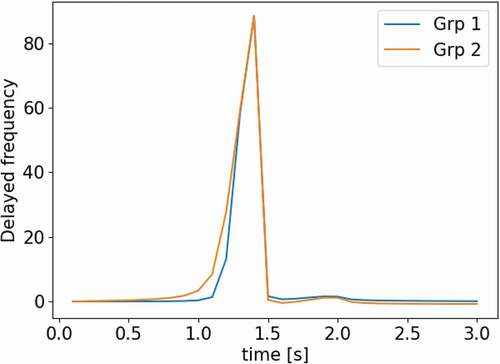
Fig. 12. Spatial distribution of delayed frequencies for precursor group 2 at different points in time, as calculated by the omega method (in units of inverse seconds).

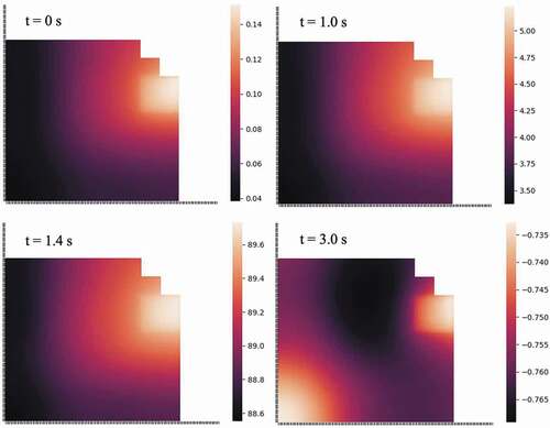
TABLE II Sensitivity of the Adiabatic Method to Outer Time Step Size

	Reference	0.01 s Outer Step Solution	0.01 s	0.05 s	0.1 s	0.5 s
			Percent Relative Difference from Reference
Time to first peak (s)	1.44545	1.4453	0.01	0.00	0.02	0.13
Power at first peak (W/cm^3)	5448.7	5338.6	2.02	1.37	1.80	0.41
Power at second peak (W/cm^3)	792.8	790.4	0.30	0.26	0.19	1.12
Power at t = 3 s (W/cm^3)	98.06	98.79	0.74	0.75	0.69	0.58

TABLE III Sensitivity of the Omega Method to Outer Time Step Size

	Reference	0.01 s Outer Step Solution	0.01 s	0.05 s	0.1 s	0.5 s
			Percent Relative Difference from Reference
Time to first peak (s)	1.44545	1.4452	0.02	0.02	0.02	0.16
Power at first peak (W/cm^3)	5448.7	5364.5	1.55	1.11	1.43	0.01
Power at second peak (W/cm^3)	792.8	792.2	0.08	0.06	0.04	1.01
Power at t = 3 s (W/cm^3)	98.06	98.90	0.86	0.87	0.84	0.61

Fig. 13. Normalized assembly power densities at the peak for adiabatic versus omega. In green and red are errors that are lower and higher for omega method, respectively.

Fig. 14. Assembly temperatures at the end of transient for adiabatic versus omega. In green and red are errors that are lower and higher for omega method, respectively.

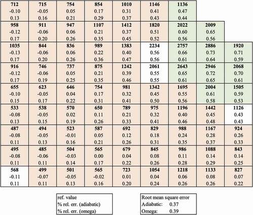
TABLE IV Alpha Eigenvalue Results, Obtained with 0.1 s Outer Time Steps

	Reference	Classic	Modified	Hybrid
		Percent Relative Difference from Reference
Time to first peak (s)	1.44545	0.02	0.02	0.02
Power at first peak (W/cm^3)	5448.7	0.16	1.47	1.42
Power at second peak (W/cm^3)	792.8	0.98	0.29	0.05
Power at t = 3 s (W/cm^3)	98.06	1.78	0.50	0.84

Fig. 15. Power profile, zoomed-in.

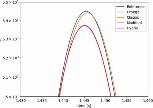
Fig. 16. Absolute error with respect to reference, in time, zoomed to the second peak.

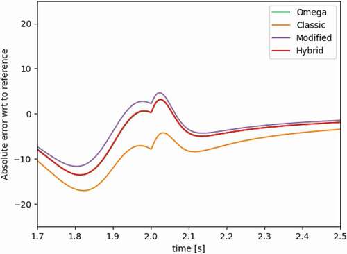
Fig. 17. Values of k-balance over time.

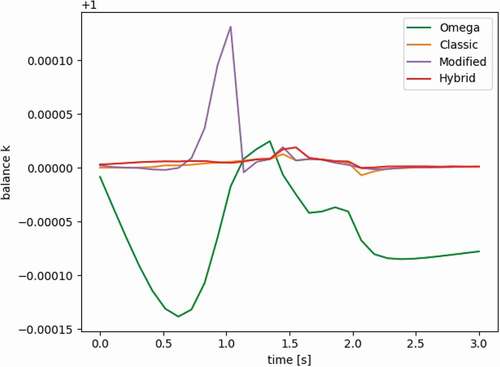
Fig. 18. Normalized assembly power densities at the peak for modified versus hybrid alpha. In green and red are errors that are lower or higher for hybrid, respectively.

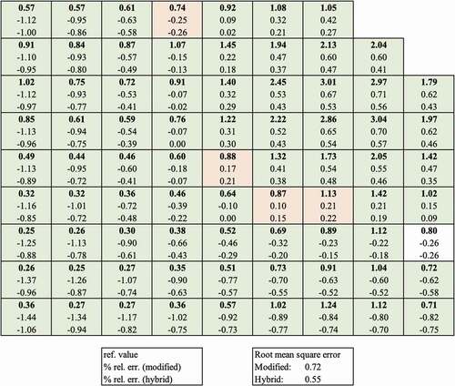
Fig. 19. Assembly temperatures at the end of transient for modified versus hybrid alpha. In green and red are errors that are lower or higher for hybrid, respectively.

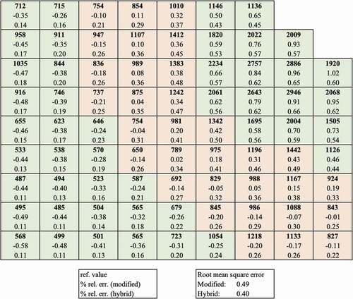
TABLE V Sensitivity of the Coarse Time Integration Method to Outer Time Step Size

	Reference	0.001 s Outer Step Solution	0.001 s	0.005 s	0.01 s
			Percent Relative Difference from Reference
Time to first peak (s)	1.44545	1.4457	0.02	0.01	0.02
Power at first peak (W/cm^3)	5448.7	5389.9	1.08	1.20	1.55
Power at second peak (W/cm^3)	792.8	791.2	0.20	0.21	0.24
Power at t = 3 s (W/cm^3)	98.06	98.27	0.21	0.21	0.21

TABLE VI Sensitivity of the Stripped-Down Coarse Time Integration Method to Outer Time Step Size

	Reference	0.001 s Outer Step Solution	0.001 s	0.005 s	0.01 s
			Percent Relative Difference from Reference
Time to first peak (s)	1.44545	1.440	0.38	2.11	4.53
Power at first peak (W/cm^3)	5448.7	5425.1	0.43	2.03	3.56
Power at second peak (W/cm^3)	792.8	794.0	0.15	0.45	0.10
Power at t = 3 s (W/cm^3)	98.06	98.01	0.05	0.25	0.50

TABLE VII Time-Differencing Results, Obtained with 0.01 s Outer Time Steps

	Reference	Coarse	IQS	FTM
		Percent Relative Difference from Reference
Time to first peak (s)	1.44545	0.02	0.14	0.09
Power at first peak (W/cm^3)	5448.7	1.55	1.58	0.94
Power at second peak (W/cm^3)	792.8	0.24	0.16	0.32
Power at t = 3 s (W/cm^3)	98.06	0.21	0.10	0.13

Fig. 20. Comparing prompt frequencies in the FTM to the amplitude derivative term in the IQS method.

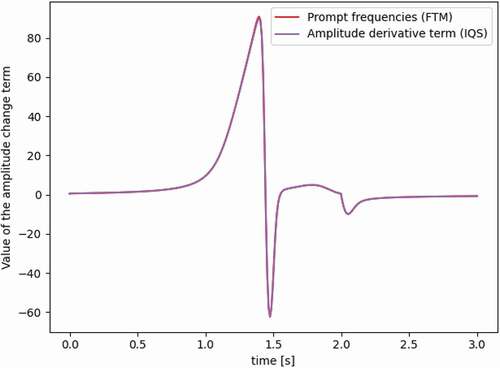
Fig. 21. Zoomed-in power profile.

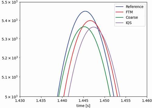
Fig. 22. Normalized assembly power densities at the peak for the IQS method versus the FTM. In green and red are errors that are lower and higher for FTM, respectively.

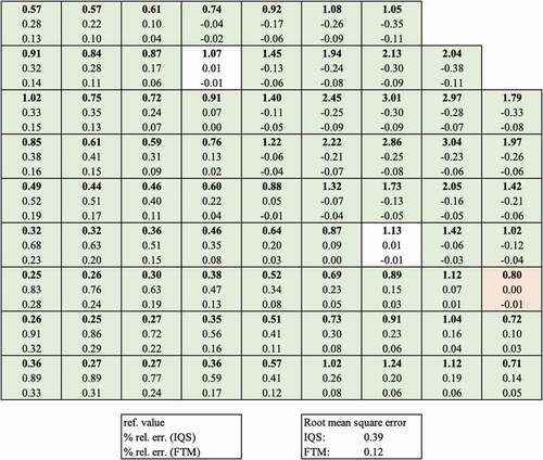
Fig. 23. Assembly temperatures at the end of transient for the IQS method versus the FTM. In green and red are errors that are lower and higher for FTM, respectively.

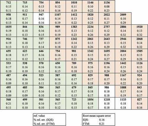
TABLE VIII Impact of Frequencies on Peak Power RMS Error

	RMS Error in Absence of Frequencies	RMS Error in Presence of Frequencies	Difference in RMS Error
k-eigenvalue methods	Adiabatic	Omega	22%
	0.79	0.57
Alpha-eigenvalue methods	Modified alpha	Hybrid alpha	17%
	0.72	0.55
Time-differencing methods	IQS	FTM	27%
	0.39	0.12

Fig. A.1. 2D-LRA geometry.¹¹

M. ABDO, R. ELZOHERY, and J. ROBERT, “Analysis of the LRA Reactor Benchmark Using Dynamic Mode Decomposition,” Trans. Am. Nucl. Soc., 119, 683 (2018).

 Google Scholar

K. SMITH, “An Analytical Nodal Method for Solving the Two Group, Multidimensional, Static and Transient Neutron Diffusion Equation,” Master Thesis, Massachusetts Institute of Technology, Nuclear Science & Engineering (1979).

 Google Scholar