Frequency-Dependent Discrete Implicit Monte Carlo Scheme for the Radiative Transfer Equation

Figures & data

Fig. 1. Low-statistic IMC and DIMC runs versus high-statistic ISMC run for (a) the material temperature at different times for the 1-D Olson³² test problem and (b) the radiation energy density at different times for the 1-D Olson³² test problem.

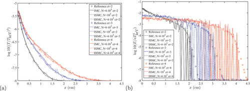
Fig. 2. Material temperature at time $t=1$ ns for the first three Densmore et al.²⁷ benchmarks: (a) ${\sigma }_0(x)=10\mathrm{k}\mathrm{e}{\mathrm{V}}^{7/2}$/cm, (b) ${\sigma }_0(x)=100\mathrm{k}\mathrm{e}{\mathrm{V}}^{7/2}$/cm, and (c) ${\sigma }_0(x)=1000\mathrm{k}\mathrm{e}{\mathrm{V}}^{7/2}$/cm.

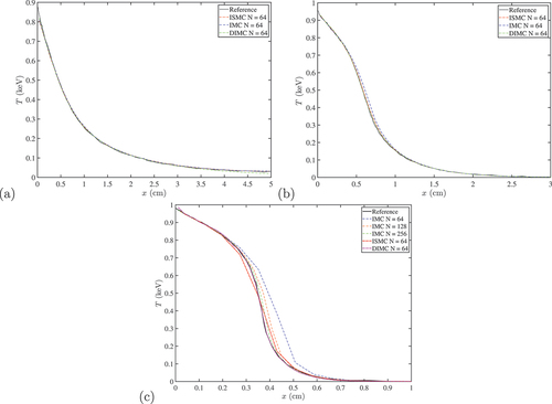
Fig. 3. Material temperature at time $t=1$ ns for the two-media Densmore et al.²⁷ benchmark: (a) zoom out showing the entire domain and (b) zoom in showing the interface between the optically thin and optically thick materials located at $x=2$ cm.

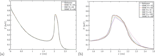
Fig. 4. Geometrical setup for the 2-D frequency-dependent benchmark of Olson.³² The gray squares represent opaque regions.

Fig. 5. (a) Contours of the logarithm of the radiation energy density at $ct=3$ using the $P_{51}$ approximation. Figure (a) is taken from Ref. 32. The radiation energy density at $ct=3$ is shown in (b) for the IMC method, (c) for the ISMC method, and (d) for the DIMC method.

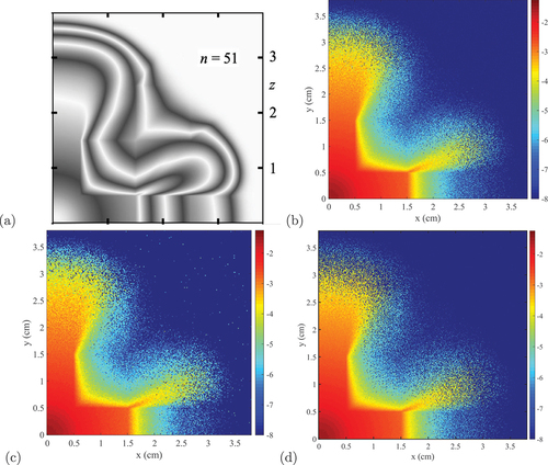
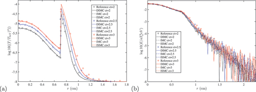
Fig. 6. (a) Material temperatures at different times for the Olson³² 2-D test problem and (b) the radiation energy density at different times for the Olson³² 2-D test problem.

G. L. OLSON, “Stretched and Filtered Multigroup Pn Transport for Improved Positivity and Accuracy,” J. Comput. Theor. Transport, 49, 5, 215 (2020); https://doi.org/10.1080/23324309.2020.1800745.

 Web of Science ®Google Scholar

J. D. DENSMORE, K. G. THOMPSON, and T. J. URBATSCH, “A Hybrid Transport-Diffusion Monte Carlo Method for Frequency-Dependent Radiative-Transfer Simulations,” J. Comput. Physics, 231, 20, 6924 (2012); https://doi.org/10.1016/j.jcp.2012.06.020.

 Web of Science ®Google Scholar