Angular Adaptivity in P⁰ Space and Reduced Tolerance Solves for Boltzmann Transport

Figures & data

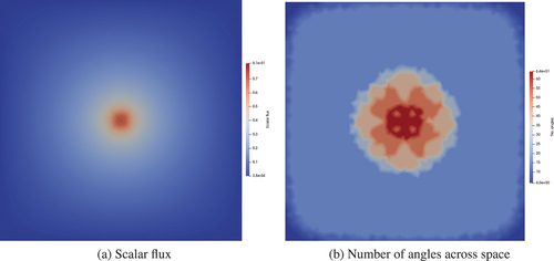
Fig. 1. Angular domains showing angular adaptivity focused around a single important direction, namely, $\mathit{\mu }\in [0,1]$ and $\mathit{\omega }\in [1.47976,1.661832]$ in a two-dimensional simulation.

Fig. 2. Sparsity of the streaming/removal operator with and without angular adaptivity, after three adapt steps. The solution of the adapted problem is shown in Fig. 4g with the spatial distribution of adapted angles shown in Fig. 4h.

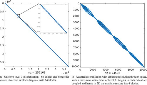
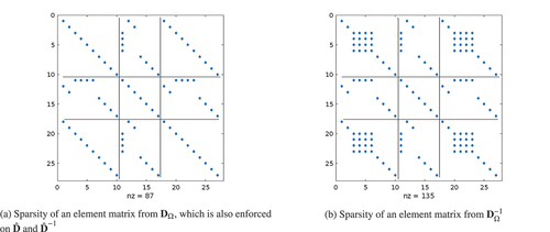
Fig. 3. Sparsity of an element streaming matrix from $\mathbf{D}$ given adapted P0 angle in 2D.

Table

Algorithm 1. METIS 5.1^[Citation36] Directional Coarsening Algorithm

1: Construct the dual-graph of the mesh

2: Construct a coarsening direction, $\mathit{a}$, at every node, by using the center of the most refined angular element

3: Compute $\mathit{s}$ to be the average scattering cross-section at every node from each of the connected elements

4: Get the number of angles on every node, $\mathit{n}$ and the number of angles with a uniform discretization, $n_{\mathit{uniform}}$

5: if $\mathit{s}>1$ or $\mathit{n}\approx n_{\mathit{uniform}}$ then

6:      Set $\mathit{a}=\mathbf{0}$ on a node

7: end if

8: Build integer area/volume weights from the dual-graph by scaling relative face areas and volumes to between 1 and 100

9: while we haven’t visited every face - denote current face as $\mathit{f}$ do

10:      Compute $a_{\mathit{avg}}$ to be the average coarsening direction on $\mathit{f}$ from each of the vertices on this face

11:      Compute $\mathit{\vartheta }$ to be the dot product between a vector parallel to $\mathit{f}$ and $a_{\mathit{avg}}$

12:      if $\mathit{\vartheta }<\mathit{\pi }/4$ and $a_{\mathit{avg}}\ne \mathbf{0}$ then

13:           Set the integer area weight on this face to be 1

14:      end if

15: end while

16: Set desired agglomerate size, $\mathit{s}$

17: Set the number of partitions as: int(number of elements/$\mathit{s}$)

18: if number of partitions $>$ 8 then

19:      Call METIS_PartGraphKway

20: else

21:      Call METIS_PartGraphRecursive

22: end if

23: Cleanup the coarsening

TABLE I Results from Using AIRG on a Pure Streaming Problem with CF Splitting by Directional Element Agglomeration

CG Nodes	Adapt Step	NDOFs	$n_{\mathit{its}}$	CC	Op Complx	WUs^full	WUs^DG	Memory
2313	1	6.3 $\times$ 10^4	17	5.1	2.7	115	27.3	10.9
2313	2	9.2 $\times$ 10^4	16	5.3	2.8	112	26.9	11.3
2313	3	2.2 $\times$ 10^5	17	5.8	3.0	128	30.5	11.9
2313	4	2.8 $\times$ 10^5	16	5.2	2.8	111	26.5	11.2
2313	5	3.1 $\times$ 10^5	19	5.3	2.8	130	31.0	11.2

Fig. 4. Adapt results for a two-dimensional pure streaming problem with a small source at the center of the domain, allowing a maximum of three levels of regular angular refinement (giving a maximum number of angles as 64). The first column shows the scalar flux, and the second column shows the number of angles across space. The third column shows the resulting element agglomeration on the second spatial grid if the directional algorithm in Sec. IV.A is used (an element coloring is used to show individual agglomerates). The rows show consecutive regular adapt steps.

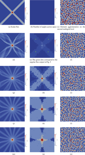
Fig. 5. Angular flux at four spatial points after two regular adapt steps in a pure streaming problem with a small source at the center of the domain. The four spatial points correspond to the green dots shown in Fig. 4e.

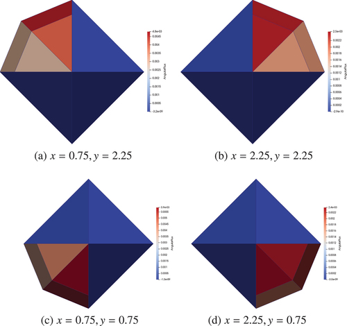
TABLE II Results from Using AIRG on a Pure Streaming Problem with CF Splitting by Falgout-CLJP

CG Nodes	Adapt Step	NDOFs	$n_{\mathit{its}}$	CC	Op Complx	WUs^full	WUs^DG	Memory
2313	1	6.3 $\times$ 10^4	9	4.4	2.87	60	14.1	10.2
2313	2	9.2 $\times$ 10^4	11	4.7	3.2	74	17.6	10.7
2313	3	2.2 $\times$ 10^5	12	5.0	3.6	85	20.2	11.3
2313	4	2.8 $\times$ 10^5	11	4.6	3.3	73	17.5	10.7
2313	5	3.1 $\times$ 10^5	11	4.5	3.2	72	17.2	10.6

Fig. 6. Field of values of the streaming operators on the third spatial grid. Blue is uniform level 3 angular refinement, and red is an adapted angular discretization with a maximum level of refinement of 3.

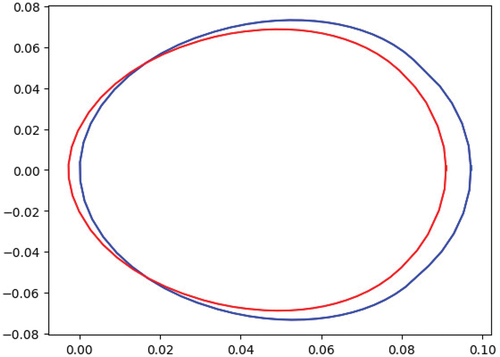
Fig. 7. Adapt results for a two-dimensional pure scattering problem with total and scatter cross sections of 10.0 with a small source at the center of the domain, allowing a maximum of three levels of regular angular refinement (giving a maximum number of angles as 64). The first column shows the scalar flux, and the second column shows the number of angles across space. The third column shows the resulting element agglomeration on the second spatial grid if the directional algorithm in Sec. IV.A is used (an element coloring is used to show individual agglomerates). The rows show consecutive regular adapt steps.

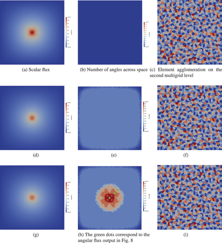
Fig. 8. Angular flux at three spatial points after three regular adapt steps in a pure scattering problem with a small source at the center of the domain. The three spatial points correspond to the green dots shown in Fig. 7h.

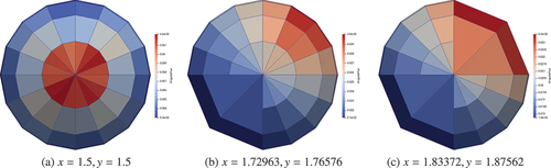
TABLE III Results from Using Additive Preconditioning on a Pure Scattering Problem with CF Splitting by Element Agglomeration

CG Nodes	Adapt Step	NDOFs	$n_{\mathit{its}}$	CC	Op Complx	WUs^mf	WUs^DG	Memory
2313	1	6.3 $\times$ 10^4	25	3.9	2.0	38	69	16.9
2313	2	2.4 $\times$ 10^5	27	3.8	2.0	39	72	16.5
2313	3	3.1 $\times$ 10^5	27	3.8	2.0	38	76	16.5

TABLE IV Results from Using Additive Preconditioning on a Pure Scattering Problem with CF Splitting by Falgout-CLJP

CG Nodes	Adapt Step	NDOFs	$n_{\mathit{its}}$	CC	Op Complx	WUs^mf	WUs^DG	Memory
2313	1	6.3 $\times$ 10^4	25	4.1	1.7	38	69	17.2
2313	2	2.4 $\times$ 10^5	27	4.0	1.4	39	73	16.5
2313	3	3.1 $\times$ 10^5	27	4.1	1.4	38	77	16.5

Fig. 9. Adapt results after five regular adapt steps in a pure streaming problem with adapt steps prior to the final step solved with wavelet-based reduced tolerance to determine convergence.

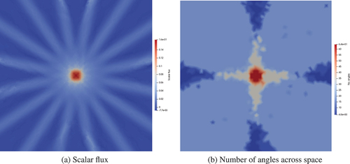
TABLE V Results from Using AIRG on a Pure Streaming Problem with CF Splitting by Falgout-CLJP with Adapt Steps Prior to the Final Step Solved with Wavelet-Based Reduced Tolerance to Determine Convergence

CG Nodes	Adapt Step	NDOFs	$n_{\mathit{its}}$	CC	Op Complx	WUs ^full	WUs^DG	Memory
2313	1	6.3 $\times$ 10^4	2	4.4	2.87	22	5.3	10.2
2313	2	9.2 $\times$ 10^4	6	4.7	3.3	47	11.3	10.6
2313	3	2.2 $\times$ 10^5	7	5.0	3.6	56	13.4	11.1
2313	4	2.8 $\times$ 10^5	7	4.6	3.3	53	12.6	10.6
2313	5	3.1 $\times$ 10^5	10	4.5	3.2	66	15.9	10.4

TABLE VI Total and Rescaled WUs from Using AIRG on a Pure Streaming Problem with CF Splitting by Falgout-CLJP*

CG Nodes	Maximum Angle Order	Uniform or Adapt	Adapt Steps	NDOF Final Adapt Step	Total WUs Rescaled
2313	3	Uniform	—	1 $\times$ 10^6	70
2313	3	Adapt	5	3.1 $\times$ 10^5	72
2313	3	Reduced tolerance adapt	5	3.1 $\times$ 10^5	54

*The WUs have been summed across all adapt steps and scaled by the nnzs in the uniform level 3 streaming/removal operator, so that the costs of uniform and adapted calculations can be compared.

TABLE VII Results from Using Additive Preconditioning on a Pure Scattering Problem with Adapt Steps Prior to the Final Step Solved with Wavelet-Based Reduced Tolerance to Determine Convergence

CG Nodes	Adapt Step	NDOFs	$n_{\mathit{its}}$	CC	Op Complx	WUs^mf	WUs^DG	Memory
2313	1	6.3 $\times$ 10^4	2	4.1	1.7	4	7.6	17.2
2313	2	2.4 $\times$ 10^5	10	4.0	1.4	16	28.8	16.2
2313	3	3.1 $\times$ 10^5	25	4.1	1.4	36	72	16.3

TABLE VIII Total and Rescaled WUs from Using AIRG on a Pure Scattering Problem with CF Splitting by Falgout-CLJP*

CG Nodes	Maximum Angle Order	Uniform or Adapt	Adapt Steps	NDOF Final Adapt Step	Total WUs Rescaled
2313	3	Uniform	—	1 $\times$ 10^6	41
2313	3	Adapt	3	3.1 $\times$ 10^5	26
2313	3	Reduced tolerance adapt	3	3.1 $\times$ 10^5	17

*The WUs have been summed across all adapt steps and scaled by the FLOPs required to compute a uniform level 3 matvec, so that the costs of uniform and adapted calculations can be compared.

Fig. 10. Adapt results after three regular adapt steps in a pure scattering problem with adapt steps prior to the final step solved with wavelet-based reduced tolerance to determine convergence.

G. KARYPIS and V. KUMAR, “Metis-Unstructured Graph Partitioning and Sparse Matrix Ordering System, Version 2.0,” University of Minnesota (1995).

 Google Scholar