Analysis of the Operational and Safety Features of the In-Core Bubbling System of the Molten Salt Fast Reactor

Figures & data

TABLE I Main Properties from the Design Specification for the MSFR

Parameter	Value
Power	3 GW(thermal)/1.5 GW(electric)
Salt volume	18 m^3
Salt fraction in core	50%
Number of circulation loops	16
Nominal flow rate	18 500 kg/s
Nominal circulation time	4.0 s
Inlet/outlet temperature	973 K/1073 K
Blanket volume	7.3 m^3

Fig. 1. Layout of the MSFR, from Ref. [16].

Fig. 2. Coupling scheme used by the solver.

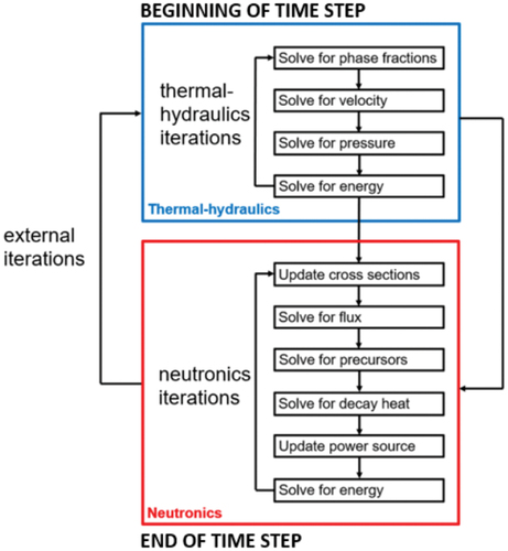
TABLE II Employed Energy Groups and Relative Coefficients for Albedo Boundary Conditions

Group	Energy MeV)	Reflector Albedo Coefficient	Blanket Albedo Coefficient
1	$2.23\mathrm{to}20.00$	$0.1455$	$0.1249$
2	$4.98\times {10}^{-1}\mathrm{to}2.23$	$0.5440$	$0.3849$
3	$2.48\times {10}^{-2}\mathrm{to}4.98\times {10}^{-1}$	$0.7771$	$0.6745$
4	$5.53\times {10}^{-3}\mathrm{to}2.48\times {10}^{-2}$	$0.7206$	$0.7596$
5	$7.49\times {10}^{-4}\mathrm{to}5.53\times {10}^{-3}$	$0.9602$	$0.8475$
6	$0\mathrm{to}7.49\times {10}^{-4}$	$1.3336$	$1.0951$

TABLE III Fission Yields at $400\mathrm{keV}$ for the Investigated Isotopes

Isotope	Fission Yield	Isotope	Fission Yield
^80Kr	$4.801\times {10}^{-8}$	^130Xe	$1.614\times {10}^{-7}$
^82Kr	$8.767\times {10}^{-7}$	^131Xe	$2.306\times {10}^{-2}$
^83Kr	$9.919\times {10}^{-3}$	^132Xe	$2.985\times {10}^{-2}$
^84Kr	$4.639\times {10}^{-2}$	^133Xe	$4.116\times {10}^{-2}$
^85Kr	$9.243\times {10}^{-3}$	^134Xe	$5.883\times {10}^{-2}$
^86Kr	$6.912\times {10}^{-2}$	^135Xe	$5.195\times {10}^{-2}$
^128Xe	$1.346\times {10}^{-6}$	^136Xe	$6.686\times {10}^{-2}$
^129Xe	$6.973\times {10}^{-9}$

TABLE IV Decay Constants for Radioactive GFPs

Isotope	Decay Constant (s^–1)
^133Xe	$1.530\times {10}^{-6}$
^135Xe	$2.107\times {10}^{-5}$

Fig. 3. (a) Geometry and (b) computational mesh employed for 2D simulations.

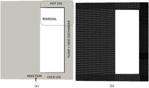
Fig. 4. (a) Geometry and (b) computational mesh employed for 3D simulations.

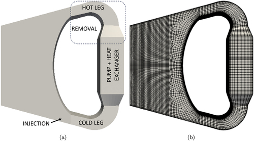
Fig. 5. Initial conditions for quantities of interest: (a) pressure, (b) temperature, (c) velocity, and (d) fission rate with the 2D geometry.

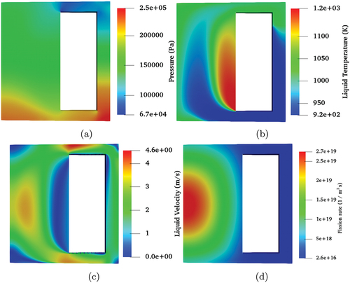
Fig. 6. Initial conditions for quantities of interest: (a) pressure, (b) temperature, (c) velocity, and (d) fission rate with the 3D geometry.

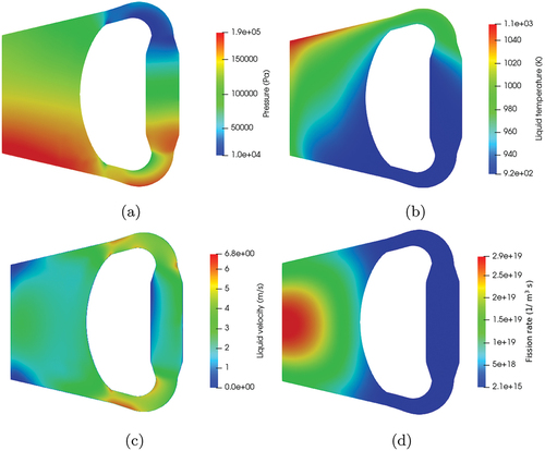
TABLE V Initial Inventories for the Various GFPs in 2D Simulations

Isotope	Initial Condition (kg)
^131Xe	$7.60\times {10}^{-3}$
^132Xe	$1.31\times {10}^{-2}$
^133Xe	$8.01\times {10}^{-3}$
^134Xe	$2.99\times {10}^{-2}$
^135Xe	$7.62\times {10}^{-4}$
^136Xe	$3.11\times {10}^{-2}$

TABLE VI Initial Inventories for the Various GFPs in 3D Simulations

Isotope	Initial Condition (kg)
^131Xe	$3.71\times {10}^{-2}$
^132Xe	$6.03\times {10}^{-2}$
^133Xe	$3.69\times {10}^{-2}$
^134Xe	$1.45\times {10}^{-1}$
^135Xe	$3.45\times {10}^{-3}$
^136Xe	$1.50\times {10}^{-1}$

Fig. 7. Initial distribution of the ¹³⁵Xe isotope in (a) 2D geometry and (b) 3D geometry.

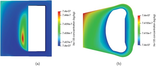
Fig. 8. Efficiency in 2D geometry: (a) time evolution of the cycle time $\mathit{\tau }$ at various helium flow rates and (b) illustration of the inverse proportionality between the cycle time $\mathit{\tau }$ and the helium flow rate. The coefficient of determination R² is 0.994 at 20 s and 0.992 at 30 s.

Fig. 9. Efficiency in 3D geometry: (a) time evolution of the cycle time $\mathit{\tau }$ at various helium flow rates and (b) illustration of the inverse proportionality between the cycle time $\mathit{\tau }$ and the helium flow rate. The coefficient of determination R² is 0.988.

TABLE VII Comparison Among Cycle Times Found in Two Dimensions and Three Dimensions*

Two Dimensions		Three Dimensions
Helium Flow Rate (g/s)	Cycle Time (s)	Helium Flow Rate (g/s)	Cycle Time (s)
0.1	97	0.1	304
0.2	56	0.3	81
0.3	32	0.5	52
0.4	26
0.5	23

*Helium flow rates refer here to the values in the simulation.

TABLE VIII Comparison Among Cycle Times Found in Two Dimensions and Three Dimensions Against the Average Helium Fraction*

Average Helium Fraction	Cycle Time (s)	Simulation
0.0047	304	3D – 0.1 g/s
0.0101	97	2D – 0.1 g/s
0.0148	81	3D – 0.3 g/s
0.0226	56	2D – 0.2 g/s
0.0242	52	3D – 0.5 g/s
0.0334	32	2D – 0.3 g/s
0.0439	26	2D – 0.4 g/s
0.0556	23	2D – 0.5 g/s

*The values in the simulation column refer to the geometry and helium flow rate used in the calculation.

Fig. 10. Graphical representation of the data reported in Table VIII.

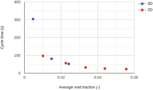
TABLE IX Contributions to Activity and Decay Heat of the Removed Gas Found with the 3D Geometry*

Isotope	Activity (Bq)	Decay Heat (W)
^133Xe	$8.85\times {10}^{17}$	$2.55\times {10}^4$
^135Xe	$1.14\times {10}^{18}$	$1.03\times {10}^5$
Total	$2.03\times {10}^{18}$	$1.28\times {10}^5$

*Values are referred to the whole core.

Fig. 11. Activity leaving the core in the gas per unit time found with the 3D geometry, referred to the whole core. Notice the logarithmic scale.

Fig. 12. Circulating delayed fraction as a function of flow rate.

Fig. 13. Power variation, void fraction, and salt temperature as functions of flow rate variation.

TABLE X Void Coefficient at Various Helium Flow Rates in 2D Geometry

Helium Flow Rate (g/s)	Void Fraction (%)	Void Coefficient ($\mathrm{pcm}/\mathrm{\%}$)
0.1	0.69	$-293$
0.2	1.8	$-245$
0.3	3.2	$-218$
0.4	5.0	$-192$
0.5	6.9	$-187$

Fig. 14. Normalized power, void fraction, and mean salt temperature after losing helium injection.

Fig. 15. Normalized power and void fraction after losing helium removal.

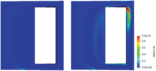
Fig. 16. Volume fraction of the gas at the beginning (left) and after 10s (right) of loss of helium removal. Notice the common scale.

M. ALLIBERT et al. “7 – Molten Salt Fast Reactors,” Handbook of Generation IV Nuclear Reactors, Woodhead Publishing Series in Energy, p. 157, I. L. PIORO, Ed., Woodhead Publishing; https://doi.org/10.1016/B978-0-08-100149-3.00007-0.

 Google Scholar

Data Availability Statement

The data that support the findings of this study are openly available in Zenodo at http://doi.org/10.5281/zenodo.7515490.