Comparison of methods for characterising the steel cleanness in powder metallurgical high-speed steels

Figures & data

Table 1. Chemical composition of the examined steel.

C [wt%]	Si [wt%]	Mn [wt%]	Cr [wt%]	Mo [wt%]	V [wt%]	W [wt%]	S [wt%]	O [wt%]
1.29	0.60	0.30	4.20	5.00	3.00	6.30	0.012	0.004

Table 2. Specifications of the CF tests.

Parameter	HCF-test	VHCF-test
Test temperature	∼23°C	∼23°C
Stress ratio	0.1	−1
Test frequency	∼158 Hz	∼965 Hz
Stress amplitude	700 MPa	820–960 MPa
Mean stress	856 MPa	0
Test arrangement	Tension arrangement	Tension compression arrangement

Figure 1. Sample geometries used in the HCF (a) and VHCF (b) tests.

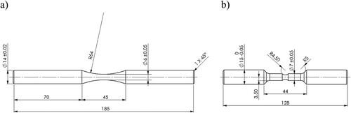
Table 3. Parameters for extraction experiments.

Specimen	Solvent	Sample shape (W x D x H)	Duration	Filter
E1	5% nital solution (sequential)	Approx. 1 × 1 × 1 cm	2 hours (15-minute sequences)	1 µm + 10 µm
E2	5% nital solution	Approx. 1 × 1 × 1 cm	5 days	1 µm + 10 µm
E3	5% nital solution	Approx. 1.5 × 1.5 × 2 cm	7 days	1 µm + 10 µm
E4	5% nital solution + 30% HCL	Approx. 1 × 1 × 1 cm	2 hr + 5 sec	1 µm + 10 µm

Table 4. Parameters for automated SEM/EDS measurements.

SEM/EDS process parameters	Numerical value
Acceleration voltage [kV]	15
Electric charge [pC]	14
Dead time [%]	34
Number of counts input [cps]	120,000
Number of counts output [cps]	78,000
Resolution [pxl]	1024
Pixel/feature [pxl]	9
Magnification [-]	130 (3-µm feature)/400 (1-µm feature)
Measurement time [s]	1
Gray value limit [-]	15,000
Gray value matrix [-]	20,000

Figure 2. Carbide and inclusion distribution of the investigated material HS6-5-3C in a SEM image captured using a backscattered electron detector.

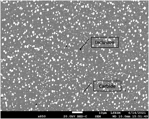
Figure 3. SEM-image in BSE-mode of a fracture-initiating inclusion on the fracture surface of a HCF specimen with corresponding EDS-elemental mappings.

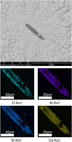
Figure 4. Relationship between the inclusion size and the load changes sustained by the samples in the HCF tests.

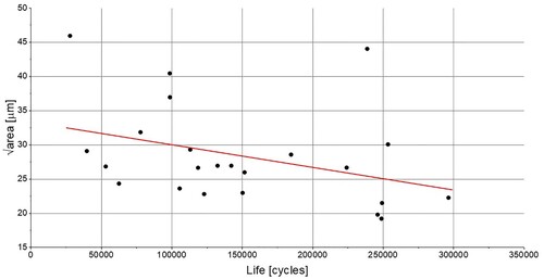
Figure 5. Applied stress amplitudes of the tests are plotted against the number of load cycles.

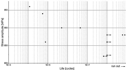
Figure 6. Relationship between the fatigue endurance strength and the inclusion size.

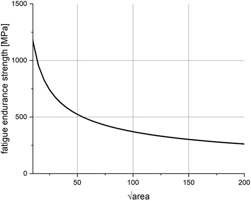
Figure 7. Box plot of sample inclusions found using light optical microscopy.

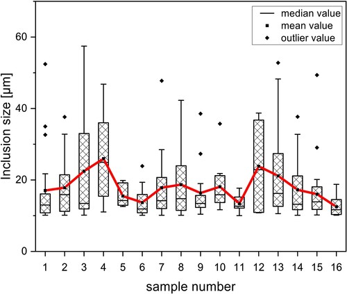
Figure 8. Log-normal distribution function of three selected specimens.

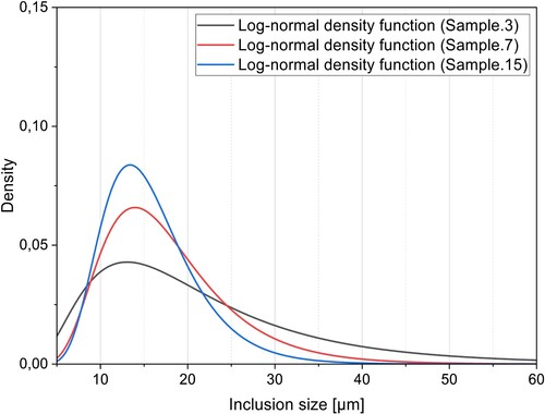
Figure 9. SEM-image in BSE-mode of oxide inclusions found on the filter after chemical extraction of specimen E3 (Duration: 7 days) with corresponding EDS-elemental mappings.

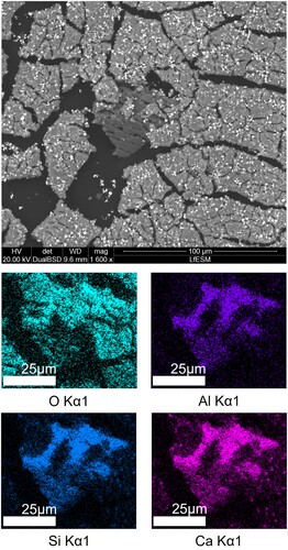
Figure 10. SEM-image in BSE-mode of oxide inclusions found on the filter after chemical extraction of specimen E1 (duration: 2 hours in 15-minute sequences) with corresponding EDS-elemental mappings.

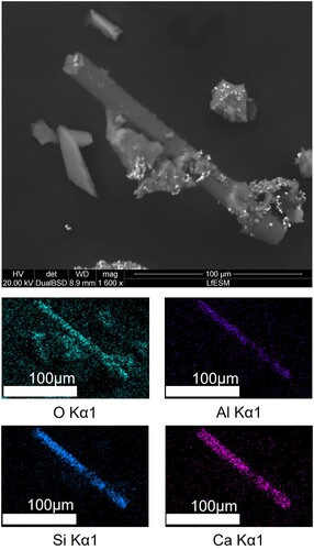
Figure 11. SEM/EDS elemental mapping of sulphide inclusions found on the filter after chemical extraction of specimen E1 (duration: 2 hours in 15-minute sequences).

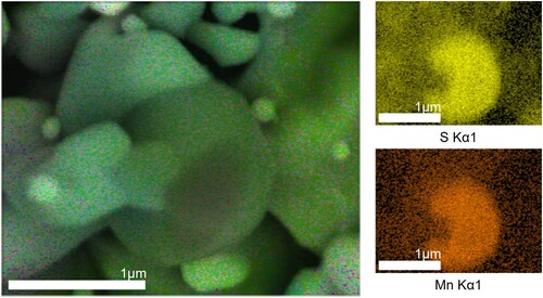
Figure 12. SEM-image in BSE-mode of oxide-sulphide inclusions found on specimen 7 with corresponding EDS-elemental mappings.

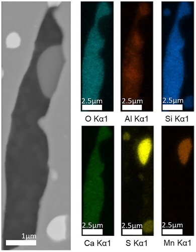
Figure 13. Composition distribution of the micro-cleanness (specimen 7).

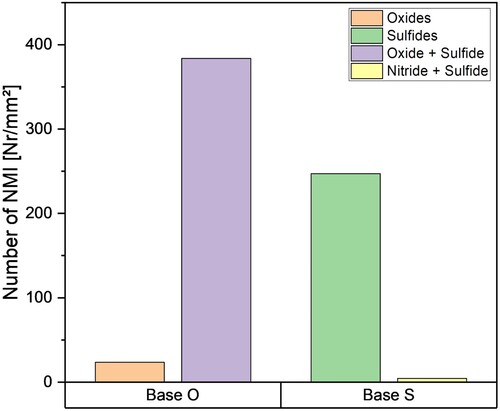
Figure 14. Comparison of inclusion composition between specimen 7 (a) and HCF samples (b) analysed with automated SEM/EDS.

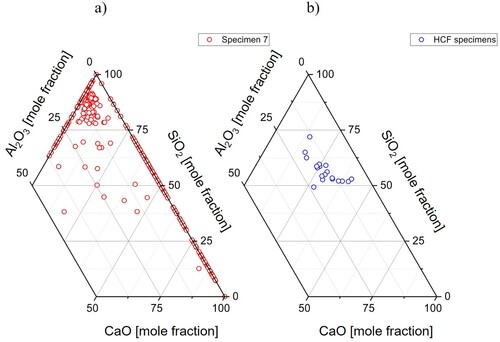
Figure 15. ME plot of specimen 7 oxide data.

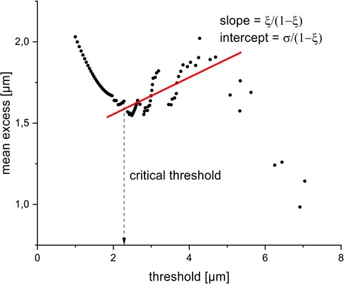
Table 5. Determined parameters of the investigated specimens.

Specimen	Type of inclusion	Shape parameters σ′	Shape parameters ζ	Inclusion density [1/mm^3]
3	Sulphides	0.114	0.121	82,986
7	Sulphides	0.143	0.044	156,295
15	Sulphides	0.108	0.102	166,813
3	Oxide–sulphides	0.199	0.097	115,117
7	Oxide–sulphides	0.482	0.035	124,730
15	Oxide–sulphides	0.175	0.123	116,348
3	Oxides	0.556	0.228	2316
7	Oxides	0.894	0.313	8738
15	Oxides	0.797	0.203	2675

Figure 16. Estimations of the largest sulphide inclusion in a given volume.

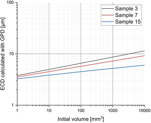
Table 6. Calculated maximum inclusion sizes of the GPD method compared with the results for the Gumbel distribution.

Inclusion group	Results GPD	Results Gumbel distribution
Oxide–sulphides	Approx. 15 µm (ECD)	Approx. 6 µm (ECD)
Sulphides	Approx. 10 µm (ECD)	Approx. 3 µm (ECD)
Oxides	Approx. 150 µm (ECD)	Approx. 13 µm (ECD)

Table 7. Method matrix with the findings from the performed analyses.

Method	Detected size	Results GPD	Detectable morphology	Detectable distribution	Detectable composition
SEM/EDS	10–100 µm	Sulphide approx. 10 µm (ECD) Oxide–sulphide approx. 15 µm (ECD) Oxide approx. 150 µm (ECD)	Yes (2D)	Yes	Yes
Manual SEM/EDS in combination with HCF	50–150 µm		Yes (3D)	No	Yes
Manual SEM/EDS in combination with extraction	10–150 µm		Yes (3D)	No	Yes
Automated SEM/EDS measurements	>1 µm		Yes (2D)	Yes	Yes
Light optical microscopy	10–50 µm		Yes (2D)	Yes	No