New region, new chances: does moving regionally for university shape later job mobility?

Figures & data

Figure 1. Selection of our sample.

Note: High schools are represented as dots. Bright (green) dots are part of the doughnut, whereas dark (red) dots are in the inner circle or outside the doughnut. The bright (green) area is the convex hull of the bright (green) schools. The inner dark (blue) area is the convex hull of the metro stations, the outer dark (blue) area is the convex hull of the suburban train stations, and the background represents the shape of the labour market region (LMR) of Munich, with the lines showing the counties within the LMR.

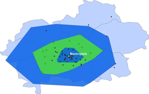
Figure 2. Overview of all Bavarian cities with a university (of applied sciences).

Note: In this map of Bavaria with county boundaries, all cities with a university (of applied sciences) are named and marked with a star. Each university (of applied sciences) is shown with a dot. The labour market region (LMR) of Munich is highlighted (in dark shading).

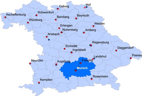
Table 1. Difference in personal characteristics between groups (defined by high-school location).

	Group of interest	Munich LMR: outside	Munich LMR: inside	Outside Munich LMR
	Mean (SD)	Mean (SD)	Mean (SD)	Mean (SD)
Parental characteristics
Mother's job qualification: low	0.13	0.18	0.19	0.20
	(0.33)	(0.39)	(0.39)	(0.40)
Mother's job qualification: medium	0.62	0.64	0.55	0.61
	(0.49)	(0.48)	(0.50)	(0.49)
Mother self-employed	0.15	0.05	0.13	0.09
	(0.36)	(0.22)	(0.34)	(0.28)
Mother's job qualification: high	0.08	0.10	0.10	0.07
	(0.27)	(0.30)	(0.30)	(0.26)
Father's job qualification: low	0.03	0.02	0.07	0.06
	(0.16)	(0.15)	(0.25)	(0.24)
Father's job qualification: medium	0.29	0.30	0.34	0.42
	(0.45)	(0.46)	(0.47)	(0.49)
Father self-employed	0.22	0.25	0.22	0.20
	(0.41)	(0.44)	(0.41)	(0.40)
Father's job qualification: high	0.45	0.39	0.35	0.29
	(0.50)	(0.49)	(0.48)	(0.45)
Mother's education: high	0.27	0.12	0.21	0.12
	(0.45)	(0.33)	(0.41)	(0.33)
Mother's education: medium	0.10	0.04	0.08	0.06
	(0.30)	(0.19)	(0.27)	(0.24)
Father's education: low	0.35	0.48	0.48	0.60
	(0.48)	(0.50)	(0.50)	(0.49)
Father's education: medium	0.18	0.16	0.17	0.16
	(0.39)	(0.37)	(0.37)	(0.36)
Father's education: high	0.45	0.30	0.33	0.22
	(0.50)	(0.46)	(0.47)	(0.41)
Observations	320	83	726	3160

Note: Values are the mean (SD) of personal characteristics.

Table 2. Regression results: ordinary least squares (OLS) and instrumental variables (IV).

	(1)	(2)	(3)	(4)	(5)	(6)
	OLS	OLS	OLS	IV	IV	IV
Moved for university	0.383***	0.383***	0.319***	1.012***	0.948***	1.318**
	(0.0823)	(0.0814)	(0.0923)	(0.365)	(0.343)	(0.565)
First stage
Distance to university				0.0182***	0.0187***	0.0159***
				(0.00577)	(0.00577)	(0.00657)
County fixed effects	×	×	×	×	×	×
Parental controls	×		×	×		×
Further controls			×			×
Observations	320	320	270	320	320	270
F-statistic				9.956	10.448	5.825

Note: Dependent variable: Moved for job. Instrument: Distance to university. Robust standard errors. All results contain fixed effects for the county. Parental control: father's occupational status (four categories). Further controls: gender, age, nationality, cohort, type of entrance diploma, high-school grade, subject of study (economics, engineering, science, remaining subjects), type of university, children, partnership, high-school grade, internship and lived abroad. Standard errors are shown in parentheses. *p < 0.1, **p < 0.05, ***p < 0.01.

Table 3. Regression results: reduced form (intention to treat).

	(1)	(2)	(3)
	Moved for first job	Moved for first job	Moved for first job
Distance to university	0.0184***	0.0177***	0.0209***
	(0.00635)	(0.00626)	(0.00725)
County fixed effects	×	×	×
Parental controls	×		×
Further controls			×
Observations	320	320	270
$R^2$	0.057	0.047	0.113

Note: Dependent variable: Moved for job. Robust standard errors. All results contain fixed effects for the county. Parental control: father's occupational status (four categories). Further controls: gender, age, nationality, cohort, type of entrance diploma, high-school grade, subject of study (economics, engineering, science, remaining subjects), type of university, children, partnership, high-school grade, internship and lived abroad. Standard errors are shown in parentheses. *p < 0.1, **p < 0.05, ***p < 0.01.

Figure 3. Exclusion restriction (with parental controls).

Note: Control variables are regressed on the instrument (distance to university). All results contain fixed effects for the county. Parental control: father’s occupational status.

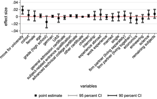
Figure 4. Robustness of estimates when changing distances of the borders.

Note: Shown is the robustness of the main effect with respect to varying the distance threshold to define the estimation sample. All results contain fixed effects for the county and controls for the father’s occupational status.

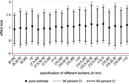
Figure 5. Robustness of estimates when controlling for different parental characteristics (broader categories).

Note: Shown is the robustness of the main effect with respect to controlling for different parental characteristics. All results contain fixed effects for the county.

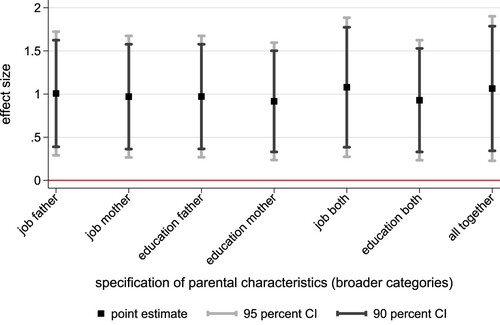
Table 4. Robustness.

Moved for first job	(1)	(2)	(3)	(4)	(5)	(6)	(7)	(8)
Moved for university	1.012***	0.574**	2.988***	1.062***	0.645**	1.270**	1.157***	1.036***
	(0.365)	(0.250)	(0.452)	(0.352)	(0.276)	(0.495)	(0.436)	(0.378)
County fixed effects	×	×	×	×	×	×	×	×
Parental controls	×	×	×	×	×	×	×	×
Return migration included		×
log Instrument								×
Probit			×
Public transport					×
Duration by car						×
Linear distance							×
Administrative approach				×
Observations	320	377	320	523	320	320	320	320
F-statistic	9.956	15.934	.	8.160	14.716	6.355	7.998	9.529

Note: Dependent variable: Moved for job. Robust standard errors. All results contain fixed effects for the county. Parental control: father's occupational status (four categories). Standard errors are shown in parentheses. *p < 0.1, **p < 0.05, ***p < 0.01.